Accelerating carbon uptake in the Northern Hemisphere: evidence from the interhemispheric difference of atmospheric CO₂ concentrations

Abstract

Previous studies have indicated that the regression slope between the interhemispheric difference (IHD) of CO₂ mixing ratios and fossil fuel (FF) CO₂ emissions was rather constant at about 0.5 ppm/Pg C yr⁻¹ during 1957–2003. In this study, we found that the average regression slopes between the IHD of CO₂ mixing ratios and IHD of FF emissions for 16 sites in the Northern Hemisphere (NH) decreased from 0.69±0.12 ppm/Pg C yr⁻¹ during 1982–1991 to 0.37±0.06 ppm/Pg C yr⁻¹ during 1996–2008 (IHD of CO₂ defined as the differences between each site and the South Pole, SPO). The largest difference was found in summer and autumn. The change in the spatial distribution of FF emissions driven by fast increasing Asian emissions may explain the slope change at three sites located north of 60°N but not at the other sites. A 30-yr SF₆ simulation with time-varying meteorology and constant emissions suggests no significant difference in the decadal average and seasonal variation of interhemispheric exchange time (τ _ex) between the two periods. Based on the hemispheric net carbon fluxes derived from a two-box model, we attributed 75% of the regression slope decrease at NH sites south of 60°N to the acceleration of net carbon sink increase in the NH and 25% to the weakening of net carbon sink increase in the SH during 1996–2008. The growth rate of net carbon sink in the NH has increased by a factor of about three from 0.028±0.023 [mean±2σ] Pg C yr⁻² during 1982–1991 to 0.093±0.033 Pg C yr⁻² during 1996–2008, exceeding the percentage increase in the growth rate of IHD of FF emissions between the two periods (45%). The growth rate of net carbon sink in the SH has reduced 62% from 0.058±0.018 Pg C yr⁻² during 1982–1991 to 0.022±0.012 Pg C yr⁻² during 1996–2008.

• CO₂
• interhemispheric difference
• carbon uptake
• carbon sink
• fossil fuel emissions
• interhemispheric exchange

To access the supplementary material to this article, please see Supplementary files under Article Tools online.

1. Introduction

During the past 30 yr, over 90% of fossil fuel (FF) CO₂ emissions have been emitted into the Northern Hemisphere (NH) and then redistributed worldwide through interhemispheric mixing on a timescale of 1–1.5 yr. In response, the atmospheric CO₂ mixing ratio in the NH has increased faster than that in the Southern Hemisphere (SH) and the interhemispheric difference (IHD) of CO₂ mixing ratios has increased from about 2 ppm in 1980 to about 3 ppm in 2003 (Keeling et al., 2011). Using regression analysis, one can decompose the IHD of CO₂ into a time-evolving component, which increases in proportion with FF emissions (i.e. the regression slope), and a time-independent regression intercept. The intercept, sometimes referred to as the stationary component of the regression (Keeling et al., 2011) given its time-independent nature, was estimated at about −1 ppm based on long-term regression analyses (e.g. Keeling et al., 1989, 2011; Conway and Tans, 1999), corresponding to a natural southward transport of around 1 Pg C yr⁻¹ across the equator. Some studies (e.g. Denning et al., 1995) suggested that an annually balanced biosphere would give rise to a positive stationary component because of the rectifier effect. However, Stephens et al. (2007) pointed out that the likelihood of a large rectifier effect was quite small. The natural ocean carbon transport – primarily in the Atlantic Ocean – was believed to be much less than 1 Pg C yr⁻¹, thus implying a stationary northern land sink (Tans et al., 1990; Fan et al., 1999; Mikaloff Fletcher et al., 2007). Keeling et al. (2011), based on atmospheric inversion, derived a larger natural ocean transport of about 0.8 Pg C yr⁻¹ southward across the equator and concluded that the stationary component could be explained only by the ocean, thus ruling out a stationary northern land sink.

The regression slope between the IHDs of CO₂ and FF emissions depends on the interhemispheric exchange time, the distribution of FF emissions and natural carbon fluxes in each hemisphere, and how the IHD of net carbon fluxes change with time, all of which may not vary in proportion with the IHD of FF emissions (defined as the NH emissions minus SH emissions). The regression slope is also affected by short-term variation in the IHD of CO₂ mainly driven by the land sink. The land sink often exhibits strong interannual variability associated with the El Niño/Southern Oscillation (ENSO) climate mode, volcanic events, and extreme weather primarily through the influence of temperature, precipitation and drought (Jones and Cox, 2001; Le Quéré et al., 2009; Zhao and Running, 2010). Previous studies (Conway and Tans, 1999; Fan et al., 1999; Taylor and Orr, 2000; Keeling et al., 2011) indicated that the regression slope was more or less stable at about 0.5 ppm/Pg C yr⁻¹ during the period 1957–2003. This is probably because the direct response of carbon sink (both land and ocean sinks here and after), such as the air-sea exchange flux and the CO₂ fertilising effect, are roughly in proportion with the growth rate of atmospheric CO₂ in both hemispheres. Recent studies indicated diverging trends of carbon sink in the NH and SH in the 2000s. Droughts may have decreased the terrestrial Net Primary Production (NPP) in the SH between 2000 and 2009 (Zhao and Running, 2010; Ahlström et al., 2012), while increasing surface wind velocities has been suggested to decrease CO₂ uptake in the Southern Ocean over the past 30 yr (e.g. Le Quéré et al., 2007; Lovenduski et al., 2008; Takahashi et al., 2009), all indicating a possible decrease of the carbon sink in the SH in the 2000s. The trend of carbon sink in the NH is more complicated. Trends of pCO₂ in the ocean suggested an increase of carbon uptake in the North Pacific Ocean, offset by a decrease in the North Atlantic Ocean since at least 1990 (e.g. Takahashi et al., 2006; Schuster et al., 2009). An increasing terrestrial NPP in the NH was suggested between 2000 and 2009 (Zhao and Running, 2010; Ahlström et al., 2012). An inventory of global established forests estimated a nearly constant northern boreal and temperate land sink of 1.2±0.1 Pg C yr⁻¹ during 1990–2007 (Pan et al., 2011). Therefore, the carbon sink in the NH has likely been stabilised or increasing during the 2000s.

Given the diverging trends of carbon sink in the NH and SH suggested by the above-mentioned studies, one would expect to see a decrease in the regression slope between the IHDs of CO₂ and FF emissions in the 2000s. In addition, Ballantyne et al. (2012) suggested a significant increase in global carbon uptake over the last 50 yr, indicating the importance of examining the change in each hemisphere. This study examines the existence of that decrease and the extent to which the variation of the IHDs of CO₂ can be used to constrain the variability of hemispheric-scale carbon sink. The time period of this analysis is from 1982 to 2008. We begin by introducing the observations and models used (Section 2). In Section 3, we apply a series of linear regressions between the IHD of CO₂ and IHD of FF emissions over the period between 1982 and 2008 to detect and quantify the slope change. In Section 4, we investigate the possible reasons for this change. We examine whether the slope change can be explained by changing spatial distribution of FF emissions or the likely underestimation of FF emissions during 1994–2007 as suggested by Francey et al. (2013). SF₆ has no known production or loss in the troposphere or stratosphere (Gloor et al., 2007; Patra et al., 2009) which makes it an ideal tracer to examine interhemispheric transport. A 30-yr simulation using SF₆ as a tracer is then used to examine whether the decadal change of interhemispheric transport can be a possible reason, followed by the analysis of the interannual variation (IAV) and the decadal-scale growth rate of the hemispheric net carbon sinks derived using a two-box model. Section 5 compares the variations of hemispheric net carbon sinks derived in this study with other studies on regional land and ocean sinks. The concluding remarks are given in Section 6.

2. Data and methods

2.1. Regression analysis

We analysed flask CO₂ measurements at 24 surface sites (16 sites in the NH and 8 sites in the SH) from the GLOBALVIEW-CO₂ network (GLOBALVIEW-CO₂, 2011), which have at most 35% internal or external gaps during the period 1982–2008 (Fig. 1 and Supplementary file). The weekly CO₂ time series at each site is fitted with a polynomial curve of degree 2 and four harmonic seasonal functions, and then lowpass-filtered with Fourier-transform ( f>0.8 cycle yr⁻¹ are removed) to derive the seasonally adjusted CO₂ time series (Thoning et al., 1989).

Fig. 1 Spatial distribution of FF CO₂ emissions for 2008 and the locations of 24 GLOBALVIEW-CO₂ sites (circles); the black boxes indicate the definition of three regions: North America (NA; 10° to 70°N, −140° to −40°E), Europe (EU; 30° to 70°N, −30° to 50°E) and Asia (AS; −11° to 55°N, 70° to 150°E).

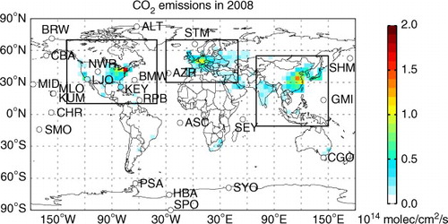
Following earlier studies (Conway and Tans, 1999; Keeling et al., 2011), we performed linear regressions between the IHD of CO₂ and the IHD of FF emissions both at monthly resolution. In this study, the IHD of CO₂ is defined as the differences in seasonally adjusted CO₂ between each site and the South Pole (SPO), in ppm. Monthly FF CO₂ emissions for 1982–2008 were taken from the 1°×1°-gridded global inventory compiled by the US Carbon Dioxide Information Analysis Center (Andres et al., 2011), which includes anthropogenic sources from solid fuels, liquid fuels, gas fuels, gas flaring and cement production in Pg C yr⁻¹. Using flask CO₂ data from the Scripps CO₂ Program in Keeling et al. (2011) (data access: http://scrippsco2.ucsd.edu/data/atmospheric_co2.html), our regression results are consistent within 1σ uncertainty with their results for all the sites except BRW (Supplementary file). The difference in BRW resulted from the lack of in situ data during 1961–1967 (Kelley, 1969) in our calculation.

2.2. SF₆ simulation and observation

GEOS-Chem (http://acmg.seas.harvard.edu/geos) is a global 3-D chemical transport model driven by Goddard Earth Observing System (GEOS) assimilated meteorology from the NASA Global Modeling and Assimilation Office (GMAO). The model version used in this study is v9-01-01. The meteorological fields are from the GMAO MERRA 30-yr reanalysis data with a native horizontal grid as fine as 0.5°×0.666° and 72 hybrid vertical grids. We simulated SF₆ at a global horizontal resolution of 4°×5° and 47 vertical levels from the surface to 0.01 hPa. The simulation was initiated from January 1979 with a global uniform SF₆ mixing ratio of 0.75 ppt, corresponding to the observed global average mixing ratio reported by Rigby et al. (2010). The model spin up was for 3 yr to get a reasonable latitudinal and vertical distribution of SF₆ (Patra et al., 2011). The distribution of SF₆ emissions in the simulation was taken from the EDGAR 4.0 (2009) gridded inventory for the period 1982–2005 (http://edgar.jrc.ec.europa.eu/part_SF₆.php). The 2005 emission distribution was used for 2006 and onwards (Fig. 2). The global total emissions of SF₆ from 1982 to 2008 were scaled to the values derived by Levin et al. (2010), which were constrained by SF₆ observations. The emission estimates by Levin et al. (2010) were verified by Rigby et al. (2010) and also demonstrated by Patra et al. (2011) to be adequate for use in independent transport models.

Fig. 2 Spatial distribution of SF₆ emissions for 2006 and the locations of 9 NOAA ESRL SF₆ observation sites (circles).

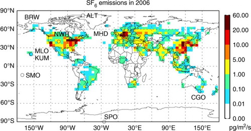
Monthly-mean observations of SF₆ at nine surface sites operated by the NOAA ESRL global monitoring division since 1995 were used for model validation (ftp.cmdl.noaa.gov,path:/hats/sf6/combined/HATS_global_SF6.txt). Flask and in situ measurements were combined to represent monthly-mean data for each site. The locations of these sites are shown in Fig. 2 and Supplementary file, including 7 background sites (ALT, BRW, MLO, KUM, SMO, CGO and SPO) and 2 northern mid-latitude sites (NWR in USA and MHD in Europe), which are closer to sources. Precision of flask and in situ SF₆ measurements at NOAA ESRL is about 0.04 ppt (1σ uncertainty). Monthly-mean model outputs were extracted for the corresponding site locations. We first corrected the vertical representativeness errors in the model for the high mountain sites, including Mauna Loa (MLO) and Niwot Ridge (NWR), the elevation of which cannot be characterised within a coarse grid of the model (Nassar et al., 2010). For example, the MLO site samples air at an elevation of 3.4 km, but the elevation of the model grid containing MLO is only 24 m since about 95% of the grid box is ocean. The modelled vertical profile of SF₆ in that grid box shows a drop of 0.07 ppt from the surface to 3.4 km (Supplementary file). To minimize the vertical sampling bias in the model, we chose the model data at higher layers instead of at the surface to match with the actual elevation of the high-elevation sites. The model output was extracted at the 18th level for MLO and the 13th level for NWR.

The time series of observed and simulated monthly-mean SF₆ at each site are fitted with a polynomial curve of degree 2 and lowpass-filtered with Fourier-transform (f>0.5 cycle yr⁻¹ are removed) to derive the long-term trend. The time derivative of the long-term trend is adopted as the growth rate of SF₆. The seasonal variation of SF₆ time series is derived from removing the long-term trend first and then highpass-filtered with Fourier-transform (f<0.8 cycle yr⁻¹ are removed).

The interhemispheric exchange time (τ _ex) can be calculated using SF₆ emissions and the hemispheric-mean mixing ratios of SF₆ using eq. (1) (Patra et al., 2009):1

where () denotes SF₆ emissions in the NH (SH), c _n (c _s ) is the hemispheric-mean mixing ratios of SF₆ in the NH (SH) in ppt, and Δc _n−s is the IHD of SF₆ in ppt. τ _ex is calculated at monthly time intervals (dt). Sensitivity tests show that the calculated τ _ex does not depend strongly on or dc _n /dt, but is sensitive to ▵c _n−s and dc _s /dt.

2.3. Two-box model of atmospheric CO₂

Equations (2) and (3) are the mass balance equations of atmospheric CO₂ in each hemisphere:2 3

where c _n (c _s ) is the hemispheric-mean mixing ratio of CO₂ in the NH (SH) in ppm, E _n (E _s ) is FF CO₂ emissions in the NH (SH) in Pg C yr⁻¹, and F _n (F _s ) is the net carbon flux (including land-use change emissions, land–air and ocean–air exchange fluxes) in the NH (SH) in Pg C yr⁻¹, and Δc _n−s is the IHD of CO₂ in ppm. The conversion factor (α) equals 2.1276 Pg C ppm⁻¹ for atmospheric CO₂ distributed globally (Sarmiento et al., 2010). To calculate the hemispheric-mean mixing ration of CO₂, we first fit a linear spline to weekly data of the 24 GLOBAIVIEW-CO₂ sites used in this study against latitude to derive the mean mixing ratio for each latitude band of 4°. The air mass-weighted average of the latitudinal-mean mixing ratios in each hemisphere is defined as the hemispheric-mean mixing ratio of CO₂.

Solving for F _n and F _s , we obtain eqs. (4) and (5):4 5

The calculation is conducted at monthly time intervals (dt). The hemispheric net carbon fluxes are seasonally adjusted with the same method as for atmospheric CO₂ in Section 2.1. All fluxes are positive into the atmosphere, so the hemispheric net carbon sinks are −F _n and −F _s .

3. Significant regression slope decrease during 1996–2008

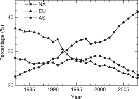
As shown in Fig. 3, the IHD of FF emissions increased rapidly by 0.11 Pg C yr⁻² during 1982–1991 and by 0.20 Pg C yr⁻² during 1999–2008, but remained relatively constant from 1992 to 1998. The slower growth rate over 1992–1998 resulted from relatively constant emissions from European countries during this period (−0.01 Pg C yr⁻²), despite a slight increase of emissions in China and Japan (by 0.05 Pg C yr⁻²). The rapid increase after 1999 is mainly driven by emissions from China and India, which have increased by 0.12 and 0.02 Pg C yr⁻², respectively. In addition to the increase of global total FF emissions, the spatial distribution of FF emissions also changed significantly, as shown in Fig. 4. The share of FF emissions from Europe (EU) in global total emissions decreased from 36.7% in 1982 to 22.3% in 2008. The share of North America (NA) was flat during 1982–2000, but decreased largely since 2001. By contrast, the share of Asia (AS) increased from 22.6% in 1982 to 41.6% in 2008. Considering the relative stabilisation of FF emissions over 1992–1998, the linear regression relationship between the IHD of CO₂ and IHD of FF emissions would be insignificant during this period. Therefore, we performed the following piecewise linear regressions for each of the 16 NH sites to identify any significant regression slope change during the period 1982–2008:6

Fig. 3 Global total (filled squares) and IHD (open circles) of FF emissions during 1982–2011. The growth rates of FF emissions during 1982–1991 and 1999–2008 are listed in the figure. The dashed lines are linear interpolated global FF emissions from 1994 to 2008.

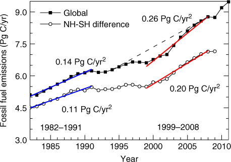
Fig. 4 The share of FF emissions from NA, EU and AS (regions defined in Fig. 1) to the global total FF CO₂ emissions during 1982–2008.

where Δc is the monthly IHD of CO₂ for each site, (E _n –E _s ) is the monthly IHD of FF emissions, Y ₁ is the ending year of the first regression period, Y ₂ is the starting year of the second regression period (Y ₂>Y ₁), α ₁ (α ₂) is the regression slope for the first (second) period, σ ₁ (σ ₂) is the corresponding ±1σ uncertainties of the regression slopes, and β ₁ (β ₂) is the regression intercept for the first (second) period. The difference in the regression slope between the two periods is defined as Δα=α ₂–α ₁. A significant slope change should meet the following three constraints: (1) p<0.05 for each linear regression; (2) ∣Δα∣>(σ ₁+σ ₂); and (3) α ₁>0, α ₂>0. Otherwise, Δα is set at zero. We also confined Y ₁≥1987 and Y ₂≤2003 in order to avoid linear regression in one period with too few data.

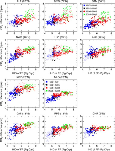
The difference in the regression slope (Δα) with different choices of Y ₁ and Y ₂ is shown in the supplementary material (Supplementary file) for all the 16 NH sites. There are five sites (CBA, SHM, AZR, BMW and KUM), which do not show any significant slope change between 1982 and 2008. At the other 11 sites, we found that Δα reached a maximum in terms of both magnitude and statistical significance when the two periods were set as 1982–1991 and 1996–2008. The scatter plots between the IHD of CO₂ and IHD of FF emissions for the 11 sites are shown in Fig. 5. The regression slopes for the two periods are clearly different at every site. Most of these sites represent the marine boundary layer, except for NWR, which shows one of the greatest changes. The choice of the two periods as 1982–1991 and 1996–2008 is consistent with the fact that the IHD of FF emissions remained relatively constant from 1992 to 1998. The open circles in Fig. 5 represent the extended data for each site. SPO has a rather intact data with gaps only between January to June 2001. There are a large number of extended data for ALT, LJO, MID, RPB and CHR at the beginning of the first period. Therefore, the regression slope at these sites may be insignificant. The GLOBALVIEW-CO₂ data are nearly intact for all the NH sites during the second period. For the 5 sites in the NH which do not show significant slope change between 1982 and 2008, three of them (CBA, SHM and KUM) are located in the Pacific Ocean and the other two (AZR and BMW) are located in the Atlantic Ocean.

Fig. 5 The scatter plots between the IHD of CO₂ and IHD of FF emissions for 11 sites in the NH. Blue and red lines are linear regression results for 1982–1991 and 1996–2008, respectively. The data for 1992–1995 are shown in black. The open squares represent the extended data for each site in GLOBALVIEW-CO₂. The green squares are the results of corrected IHD of CO₂ for 2005–2008 which eliminate the influence of the change in the spatial distribution of FF emissions.

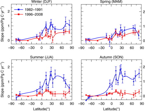
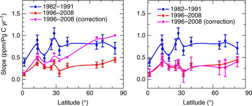
The regression slope, intercept and their uncertainties of the 11 sites in the NH and 7 sites in the SH are displayed in Fig. 6 as a function of latitude for the two selected periods: 1982–1991 (blue line) and 1996–2008 (red line). ASC and CGO in the SH have significantly negative regression slopes during the first period (ASC: −0.42±0.06; CGO: −0.29±0.04 ppm/Pg C yr⁻¹) which are not shown in Fig. 6. Conway and Tans (1999) also found a negative slope of −0.30 for ASC during 1980–1997, for which the underlying regional processes remained unknown. CGO has the extended data from January 1982 to March 1984, which are at the beginning of the first period and may affect the regression slope significantly. The magnitude of the slope difference in the NH can reach up to 0.7 ppm/Pg C yr⁻¹. The mean regression slopes for the 16 NH sites decreases from 0.69±0.12 ppm/Pg C yr⁻¹ in the first period to 0.37±0.06 ppm/Pg C yr⁻¹ in the second period, while the intercept increases from −0.68±0.58 to 1.09±0.36 ppm. We further compared the regression slopes for the two periods by season (Fig. 7). Here, winter is defined as the period from December of the previous year to February of that year. Spring, summer and autumn refer to the periods of March–May, June–August and September–November, respectively. Larger slope change is found in summer and autumn, while very little change is found in winter and spring.

Fig. 6 Regression slopes and intercepts between the IHD of CO₂ and IHD of FF emissions plotted as a function of latitude. The error bars represent ±1σ uncertainties of slopes and intercepts. The solid lines are results smoothed by a B-spline fit. The blue and red lines are results for 1982–1991 and 1996–2008 in this study. The black line is result from Keeling et al. (2011). The pink point is result from Fan et al. (1999).

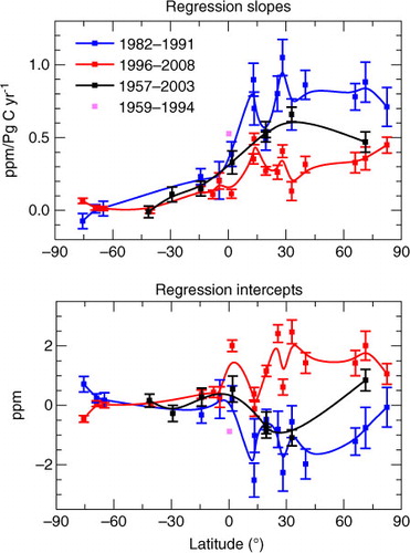
Fig. 7 Regression slopes between the IHD of CO₂ and IHD of FF emissions in each season for 1982–1991 (blue) and 1996–2008 (red).

To compare with the previous studies, Fig. 6 also presents the regression slope at eight sites (NZD, KER, SAM, CHR, KUM, MLO, LJO and BRW) for the period 1957–2003 which were reported by Keeling et al. (2011) (black line) and the regression slope at MLO for the period 1959–1994 from Fan et al. (1999) (pink point). In our study, the IHD of CO₂ is regressed against the IHD of FF emissions rather than global total emissions as in Keeling et al. (2011) and Fan et al. (1999). We regressed the IHD of CO₂ against the global total FF emissions and found small changes in regression slope (differences being 0.004±0.010 and 0.024±0.017 ppm/Pg C yr⁻¹for 1982–1991 and 1996–2008, respectively). At these common sites, our regression slopes during the first period are consistent with those derived by those two studies. Although the study period of Keeling et al. (2011) covers 8 yr (1996–2003) during which we found a significant slope change compared to the first period, it is a relatively short-term variation compared to the 47 yr’ worth of data used in their study.

4. Explanations for the significant slope decrease

First, the change in regression slope may be caused by the fact that the IHD of FF emissions is derived using hemispheric-mean FF emissions, which do not account for the influence of changing spatial distribution of FF emissions on atmospheric CO₂ mixing ratios at individual sites. As shown in Figs. 3 and 4, the rapid growth of FF emissions during 1996–2008 was mainly driven by Asia, and Asian emissions are at lower latitudes than those from UA and EU. We expect that the change in the spatial distribution of FF emissions may decrease the regression slope during the second period. Second, as our regression analysis relies on FF CO₂ emission data, the slope change could be an artifact of a change in the accuracy level of the emission data between the two periods. Francey et al. (2013), through analysis of the growth rate and IHD of atmospheric CO₂ during 1992–2011, found a clear response in atmospheric CO₂ coinciding with the sharp 2010 increase in Asian emissions but a persistently slow mean CO₂ growth from 2002/03. They suggested a cumulative underestimation of about 9 Pg C FF emissions between 1994 and 2007, which may affect our regression slope during the second period.

In the two-box model described in Section 2.3, the difference between eqs. (2) and (3) gives:7

Therefore, a slope decrease between the IHD of CO₂ and IHD of FF emissions can also be explained by the changes in the decadal average of interhemispheric exchange time (τ _ex) and/or the change in the IHD of net carbon fluxes (F _n −F _s ) relative to the IHD of FF emissions. These three possible reasons are discussed separately in this section.

4.1. FF emissions

To test whether the change in the spatial distribution of FF emissions can have a large impact on the IHD of atmospheric CO₂ mixing ratios, we conducted a standard and sensitivity simulation of CO₂ using the GEOS-Chem global chemical transport model (v9-01-03) driven by the MERRA reanalysis meteorology during 2005–2008 with a horizontal resolution of 4°×5°. The standard simulation adopts the monthly 1°×1° gridded global inventory of FF CO₂ emissions from 2005 to 2008 as described in Section 2.1. The sensitivity simulation has the same global total FF CO₂ emissions as the standard simulation, yet adopts the average spatial distribution of FF emissions during 1982–1991. CO₂ fluxes from biomass burning, biofuel burning, ocean and terrestrial biospheric exchange are taken from the work of Nassar et al. (2010) and do not differ between the two simulations. Therefore, the difference in atmospheric CO₂ between the sensitivity and standard simulation reflects the sole influence of spatial distribution changes of FF emissions.

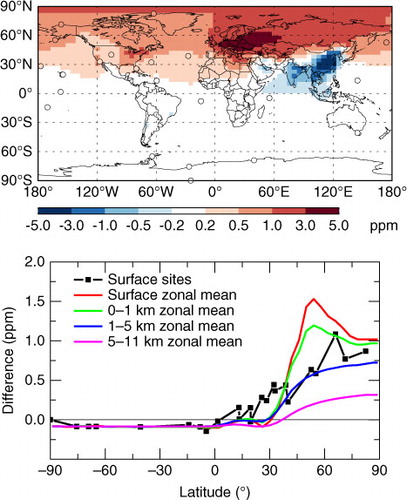
The upper panel of Fig. 8 shows the mean difference in surface CO₂ between the sensitivity and standard simulation. Compared with the standard simulation, the larger share of FF emissions over Europe in the sensitivity simulation caused dramatic increases of surface CO₂ over Europe and an overall increase greater than 0.5 ppm over 45°–90°N. The smaller share of FF emissions for Asia in the sensitivity simulation caused only decrease of surface CO₂ in East China and India. The bottom panel of Fig. 8 shows the zonal-mean difference of simulated CO₂ at the surface, 0–1, 1–5 and 5–11 km between the sensitivity and standard simulation, respectively. Although there is little change in surface CO₂ over 0–30°N in terms of zonal mean, the surface sites show an increase of 0–0.5 ppm in the sensitivity simulation because of their sample locations. The difference increases northward and reaches a maximum around 50°N at the surface. The difference decreases with altitude and shows a similar latitudinal pattern as the surface.

Fig. 8 The average difference in atmospheric CO₂ between the sensitivity and standard simulation (sensitivity minus standard) for 2005–2008. Upper panel: the spatial distribution of the difference in surface CO₂ (circles indicate the location of surface sites in this study); Bottom panel: the zonal-mean difference of CO₂ at the surface, 0–1 km, 1–5 km and 5–11 km.

To account for the impact of changing spatial distribution of FF emissions, the IHD of CO₂ mixing ratio between 2005 and 2008 is corrected by adding the difference between the sensitivity and standard simulation. The scatter plots between the corrected IHD of CO₂ and IHD of FF emissions for 2005–2008 are shown as green squares in Fig. 5. The regression slopes during the second period are recalculated using the corrected IHD of CO₂ for 2005–2008 and the same starting point as the previous regression. The results are shown in the left panel of Fig. 9. Compared with Fig. 6, the largest difference in the regression slope during 1996–2008 occurs at sites located north of 60°N (ALT, BRW and STM). The slope decreases for the three sites disappear after the correction. For sites located between 0 and 45°N, the slope decreases are still significant even after the correction.

Fig. 9 Comparisons of the corrected regression slopes with those shown in Fig. 6 (blue and red lines) in the NH. Left panel: regression slopes using the corrected IHD of CO₂ which eliminate the influence of the change in distribution of FF emissions (pink line); Right panel: regression slopes using the linearly interpolated global FF emissions from 1994 to 2008 as shown in Fig. 3 (pink line).

To examine whether the possible underestimation of FF emissions suggested by Francey et al. (2013) can affect the regression slopes during 1996–2008, we regressed the IHD of CO₂ mixing ratio with linearly interpolated global FF emissions during 1994–2008 (Fig. 3). As shown in the right panel of Fig. 9, the regression slopes during 1996–2008 do not show any significant change throughout the sites in the NH compared to Fig. 6. This indicates that the slope decrease found in this study cannot be explained by the possible underestimation of FF emissions from 1994 to 2007.

4.2. Interhemispheric exchange time

As described in Section 2.2, the GEOS-Chem SF₆ simulation driven by the MERRA 30-yr reanalysis meteorology is used to examine any significant change in τ _ex between the two periods 1982–1991 and 1996–2008. The simulation is evaluated using the global SF₆ observations from 1996 to 2008, as shown in Table 1 and in Supplementary file. The simulated SF₆ time series are in good agreement with those observed in terms of magnitude, growth rate and seasonal variation. The nine sites are representative of the zonal mean at their locations. The decadal averages of observed and simulated τ _ex during 1982–1991 and 1996–2008 are shown in Fig. 10. The calculation of τ _ex depends on the methods of deriving the hemispheric-mean mixing ratios of SF₆. For comparison between model and observation, the hemispheric-mean SF₆ is calculated from averaging the six sites in the NH and three sites in the SH (the ‘nine sites’ case in Fig. 10). The difference of observed and simulated τ _ex during 1996–2008 is 0.06 yr and within 1σ uncertainty of the observation. In the ‘nine sites’ case, the difference of simulated τ _ex between 1982–1991 and 1996–2008 is 0.05 yr. The hemispheric-mean mixing ratios are also calculated from averaging all model surface grids in the NH and SH, referred to as the ‘All grids’ case in Fig. 10. The resulting τ _ex is similar to that of the ‘9 sites’ case for both periods, suggesting again that the nine sites are representative of the hemispheric averages. The difference of simulated τ _ex between the two periods is 0.04 yr in the ‘All grids’ case. A CTM intercomparison experiment, TransCom-CH₄ (Patra et al., 2011), reported an average τ _ex of 1.3 yr during 1999–2007 for the GEOS-Chem model, which is comparable to that of 1.29 yr derived in this study. Furthermore, the GEOS-Chem model was found to fall in the middle range of τ _ex among all the models participating in TransCom-CH4 and agree well with observed τ _ex (Patra et al., 2011).

Fig. 10 Decadal averages of observed and simulated τ _ex for 1982–1991 and 1996–2008 for three cases with different calculation of hemispheric-mean mixing ratios and emission scenarios: (1) ‘9 sites’ case: average of 6 sites in the NH and 3 sites in the SH, EDGAR4.0/Levin; (2) ‘All grids’ case: average of all surface NH and SH grids, EDGAR4.0/Levin; and (3) ‘All grids_C’ case: average of all surface NH and SH grids, EDGAR_Y1980.

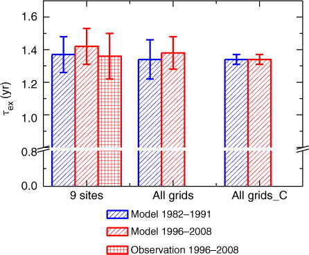
Table 1. The biases and correlations between monthly simulated and observed SF₆ at 9 NOAA observation sites during 1996–2008

Sites	ALT	BRW	MHD*	NWR	MLO	KUM	SMO	CGO	SPO
Model bias (ppt)	0.044	0.022	0.042	0.041	−0.016	−0.010	0.005	0.004	0.006
Growth rate correlation	0.94	0.96	0.79	0.93	0.95	0.93	0.93	0.86	0.75
Seasonal variation correlation	0.49	0.54	0.26	0.26	0.35	0.23	0.50	0.26	0.15

*The MHD observation data for 1996.01–1998.11 were calculated from corresponding BRW observation plus simulated difference of MHD with BRW.

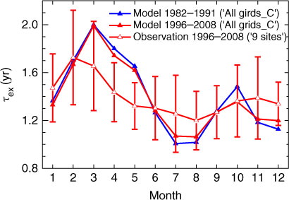
The annual observed and simulated τ _ex is shown in Fig. 11. The interannual correlation between observed and simulated τ _ex is 0.71 between 1996 and 2008. The simulated τ _ex shows an apparent increasing trend over 1982–1991 but a decreasing trend over 1996–2008. We found that the trends in τ _ex are caused by the shifts in emission distributions adopted in the simulation and this has been reported by Patra et al. (2011). The trend in τ _ex disappears when the model was driven by constant emissions for 1980. The simulation with constant emissions (the ‘All grids_C’ case in Figs. 10 and 11) reduces the IAV of τ _ex and also its difference in the decadal average between the two periods. In the ‘All grids_C’ case, there is no difference in the simulated τ _ex during the two periods (Fig. 10). According to eq. (7), a slope decrease from 0.69±0.12 to 0.37±0.06 ppm/Pg C yr⁻¹ (Section 3) requires a decrease of average τ _ex by about 0.6 yr during 1996–2008 compared to 1982–1991, which is a factor of 10 larger than the simulated difference in τ _ex by the model during the two periods. Therefore, we conclude that it is unlikely that interdecadal change or intradecadal trend in interhemispheric exchange over the two periods can explain the regression slope change presented above. Fig. 12 shows that the seasonal variation of simulated τ _ex over the two periods is also similar. Therefore, the larger slope change in summer and autumn should be mainly related with the carbon sink. However, this is not consistent with Piao et al. (2008), which suggested that the net carbon loss of northern ecosystems in response to autumn warming offset the increasing carbon uptake in the spring during 1980–2002. In the following calculation of hemispheric net carbon fluxes, we use the simulated τ _ex derived from the ‘All grids_C’ case.

Fig. 11 Annual observed and simulated τ _ex (solid lines) in the three cases in Fig. 10. The dashed lines are the linear trends of simulated τ _ex for 1982–1991 and 1996–2008.

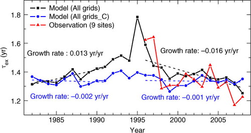
Fig. 12 Seasonal variation of observed (‘9 sites’ case) and simulated (‘All grids_C’ case) τ _ex for 1982–1991 and 1996–2008.

4.3. Hemispheric net carbon fluxes

After excluding the change in interhemispheric exchange time as a cause for the regression slope decrease, we seek to quantify the change in the IHD of net carbon fluxes and to separate the NH and SH fractions of that change which may be responsible for the regression slope decrease.

The monthly net carbon fluxes (seasonally adjusted) in the NH and SH (i.e. F _n and F _s ) from 1982 to 2008, derived using the two-box model introduced in Section 2.3, are shown in Fig. 13 (black solid lines). The derived decadal average of F _n during 2000–2008 is −2.6±0.8 Pg C yr⁻¹. By comparison, a forest inventory study (Pan et al., 2011) reported a sink of 1.2±0.1 Pg C yr⁻¹ for the boreal and temperate NH land during 2000–2007. Takahashi et al. (2009), based on pCO_2, reported a temperate and high-latitude NH ocean sink of 1.0±0.3 Pg C yr⁻¹ for the nominal year of 2000. The derived decadal average of F _s during 2000–2008 is −0.7±0.6 Pg C yr⁻¹, which can be compared with the temperate SH and Southern Ocean sink of 1.1±0.3 Pg C yr⁻¹ for the nominal year of 2000 suggested by Takahashi et al. (2009). The F _n and F _s derived in our study can also be compared with the optimised surface fluxes calculated from two atmospheric inversion studies: the NOAA Carbon Tracker (http://carbontracker.noaa.gov) and CarboScope (http://www.carboscope.eu/). These two inversion studies report the extra-tropical northern, tropical and extra-tropical southern fluxes, rather than the hemispheric-mean fluxes. Previous studies indicated that the net tropical land flux (including tropical land-use change emissions and land–air exchange flux) was nearly zero (Pan et al., 2011) and the tropical ocean flux was dominated by the SH (Takahashi et al., 2009). Therefore, we adopted the extra-tropical northern flux from the inversions for comparison with F _n and the sum of tropical and extra-tropical southern flux for comparison with F _s . The hemispheric fluxes from the inversions and this study are comparable in magnitude and the temporal correlation coefficients are above 0.7 for both hemispheres (Supplementary file).

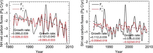
Fig. 13 Monthly net carbon fluxes (seasonally adjusted) in the NH (left panel) and SH (right panel). Black lines are the originally calculated fluxes with the two-box model (F _n and F _s ). Red lines are EVI-filtered fluxes after removal of the ENSO-Volcano related IAV in the original calculated fluxes (F _n ′ and F _s ′). The dashed lines are the linear trends for 1982–1991 and 1996–2008. Mean values and ±2σ uncertainties of the growth rate for each period are listed in the figure in Pg C/yr². Negative values indicate net carbon sink.

As shown in Fig. 13, the net carbon fluxes in both hemispheres (F _n and F _s ) exhibit increasing trends which are significant above the 2σ uncertainty during 1982–1991 and 1996–2008. Besides, both F _n and F _s show large interannual variability. The IAV of F _n relates closely with both fire emissions (R=0.79) and terrestrial NPP (R=−0.63), while the IAV of F _s relates better with terrestrial NPP (R=−0.66) but not with fire emissions (Supplementary file). We removed the long-term trend with a polynomial curve of degree 2 to obtain the IAV of each time series. Therefore, the IAV of net carbon fluxes is mainly associated with the net land fluxes which include terrestrial NPP, heterotrophic respiration and land-use change emissions.

The left panel of Fig. 14 shows the linear regression between the IHD of net carbon fluxes (F _n –F _s ) and IHD of FF emissions (E _n –E _s ). We denote the regression slope here as ΔIHD _F /ΔIHD _E , representing the ratio between the IHD of net carbon fluxes and IHD of FF emissions. As we define the fluxes as positive if into the atmosphere and negative if uptake, (F _n –F _s ) is generally negative and (E _n –E _s ) is positive. Therefore, a negative (positive) ΔIHD _F /ΔIHD _E indicates that the IHD of net carbon sink increases (decreases) with the IHD of FF emissions. The value of ΔIHD _F /ΔIHD _E is found to change significantly from +0.24±0.11 during the first period to −0.41±0.10 during the second period, suggesting a significant intensification of the IHD of carbon sink during the second period. This apparent change can be a plausible reason to explain the regression slope decrease in Section 3. However, we should note that the large IAV in F _n and F _s may affect the decadal-scale regression analysis. For example, the mean ΔIHD _F /ΔIHD _E during 1982–1991 is largely affected by the strong net carbon sink in 1991 which may be due to the eruption of Mt. Pinatubo. Therefore, in the next section we attempt to remove the impact of some known climatic and geological factors with large interannual variability on F _n and F _s . This process is referred to as filtering of hemispheric net carbon fluxes.

Fig. 14 Linear regressions between the IHD of net carbon fluxes (left panel: original calculation; right panel: EVI-filtered) and IHD of FF emissions during 1982–1991(blue) and 1996–2008 (red). The data for 1992–1995 are shown in black.

4.4. Filtering of hemispheric net carbon fluxes

We selected four climate and geological indices, including the ENSO-Volcanic index (EVI), temperature, precipitation and Palmer Drought Severity Index (PDSI). The data sources are summarised in Supplementary file. The IAV of these time series were derived after removal of the long-term trend by fitting with a polynomial curve of degree 2 and then removal of the seasonal cycle by lowpass-filtered with Fourier-transform (f>0.8 cycle yr⁻¹). Following the method described in Raupach et al. (2008), we first calculated the lagged correlation between the IAV of F _n/s (denoted as ‹F _n/s ›) and ENSO (shown in Supplementary file). The EVI in each hemisphere is then determined by:8

where τ is the ENSO lag time which maximises the correlation between ‹F _n/s › and ENSO, and λ is chosen to maximise the correlation between ‹F _n/s › and EVI. The global Volcanic Aerosol Index (VAI) data up to 1998 are adopted from ftp://ftp.ncdc.noaa.gov/pub/data/paleo/climate_forcing/volcanic_aerosols/ammann2003b_volcanics.txt, which are extended to 2008 assuming no volcanic activity between 1998 and 2008. The resulting EVI can explain 64 and 78% of the interannual variability in F _n and F _s , respectively. The lagged correlations between ‹F _n/s › and the other three indices are also shown in Supplementary file. We found that the IAV in both F _n and F _s relate most closely with EVI. Therefore, EVI was used to remove the interannual variability in F _n/s . The EVI-filtered IAV of hemispheric net carbon fluxes (denoted as ‹F _n/s ′›) is calculated using:9

where µ is chosen to minimise the variance of ‹F _n/s ′›.

‹F _n/s ′› plus the long-term trend of F _n/s gives the EVI-filtered hemispheric net carbon fluxes (F _n/s ′) (red solid lines in Fig. 13). The EVI-filtering process significantly reduces the change of F _n and F _s in 1983, 1987 and 1998 which were strong El Niño years, and the change of F _n in 1991 associated with the eruption of Mt. Pinatubo.

The right panel of Fig. 14 shows the linear regressions between the IHD of EVI-filtered hemispheric net fluxes (F _n ′−F _s ′) and the IHD of FF emissions (E _n −E _s ) for the two periods, with the regression slopes denoted as ΔIHD _F′/ΔIHD _E . The regression slopes in Fig. 14 become more statistically significant after the EVI-filtering process. During 1982–1991, the absolute magnitude of (F _n ′−F _s ′) remains more or less constant even though (E _n −E _s ) increases, with a small positive ΔIHD _F′ /ΔIHD _E of +0.11±0.08. This is consistent with the conclusion in Conway and Tans (1999) that any trend in carbon sink was small relative to the trend in FF emissions during the period 1957–1990. During 1996–2008, however, the absolute magnitude of (F _n ′−F _s ′) increases as (E _n −E _s ) increases, with a significantly negative ΔIHD _F′/ΔIHD _E of −0.36±0.09, suggesting a significant increase in the IHD of net carbon sink during the second period. The significant change of ΔIHD _F′/ΔIHD _E from +0.11±0.08 in the first period to −0.36±0.09 in the second period is responsible for the significant decrease in the regression slope presented in Section 3.

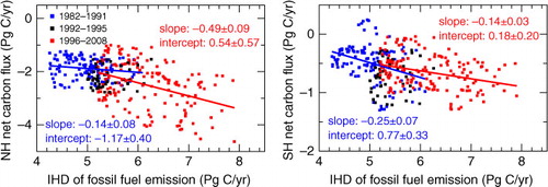
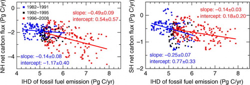
Figure 15 shows the linear regressions between the EVI-filtered hemispheric net carbon fluxes in the NH (F _n ′, left panel) and SH (F _s ′, right panel) and the IHD of FF emissions (E _n −E _s ) for 1982–1991 and 1996–2008. The regression slope between F _n ′ and (E _n −E _s ), ΔF _n ′/ΔIHD _E , changes from −0.14±0.08 in the first period to −0.49±0.09 in the second period. Although the net carbon sinks in the NH have increased in both periods as FF emissions increase, as indicated by the negative sign of the ΔF _n ′/ΔIHD _E , the growth rate of net carbon sink in the NH during the second period is much larger than that during the first period. The change in ΔF _n ′/ΔIHD _E accounts for 75% of the change in ΔIHD _F′/ΔIHD _E between the two periods presented above. The remaining 25% of the change is attributed to the change in the regression slope of F _s ′ with (E _n –E _s ) (i.e. ΔF _s ′/ΔIHD _E ) which changes from −0.25±0.07 in the first period to −0.14±0.03 in the second period. The negative sign of the ΔF _s ′/ΔIHD _E in both periods suggests an increase in the SH sinks with increasing FF emissions, while the decrease in the absolute magnitude of ΔF _s ′/ΔIHD _E in the second period indicates a weakening in the SH sinks increase relative to that of FF emissions.

Fig. 15 Linear regressions between the EVI-filtered hemispheric net carbon fluxes (F _n ′ and F _s ′) and the IHD of FF emissions for 1982–1991(blue) and 1996–2008 (red). The data for 1992–1995 are shown in black. The left panel shows the NH data and the right panel shows the SH data.

5. Discussion

The value of ΔIHD _F′/ΔIHD _E is approximately equivalent to the ratio between the growth rate of (F _n ′−F _s ′) and the growth rate of (E _n −E _s ). Figure 13 also shows the mean value and 2σ uncertainties of the growth rates for originally calculated and EVI-filtered hemispheric net carbon fluxes. The growth rate of (E _n −E _s ) during 1996–2008 is 0.16 Pg C yr⁻², which is 45% higher compared to that of 0.11 Pg C yr⁻² during 1982–1991. Net carbon sink in the NH (−F _n ′) shows an increase during 1996–2008 at a rate of 0.093±0.033 Pg C yr⁻², which is about a factor of three larger than its growth rate during 1982–1991 (0.028±0.023 Pg C yr⁻²) and exceeds the percentage increase in the growth rate of FF emissions (E _n −E _s ). In contrast, the growth rate of net carbon sink in the SH (−F _s ′) shows a reduction of 62% from 0.058±0.018 Pg C yr⁻² during 1982–1991 to 0.022±0.012 Pg C yr⁻² during 1996–2008.

There are several previous studies analysing the growth rate of the regional land and ocean sinks during the second period but debates exist for both direction and magnitude compared with those found in our study. In the NH, an increase in the land carbon sink during 2000–2009 has been suggested by the trend of terrestrial NPP. Zhao and Running (2010) estimated a mean annual growth rate of 0.128 Pg C yr⁻² during 2000–2009 for terrestrial NPP in the NH. However, Ahlström et al. (2012) estimated a much larger annual increase rate of 0.33 Pg C yr⁻² during the same period. Terrestrial NPP is only part of the land flux and there is no available study about heterotrophic respiration on the hemispheric and decadal scale. By comparison, the annual rate of increase in (−F _n ′) during 2000–2008 in our study is 0.208±0.051 Pg C yr⁻². Schuster and Watson (2007) suggested that the uptake of North Atlantic between 20°N and 65°N declined by ~0.24 Pg C yr⁻¹ from the mid-1990s to early-2000s. However, Ullman et al. (2009) argued that the North Atlantic carbon sink increased between the mid-1990s and the mid-2000s based on a biogeochemical general circulation model. The increasing trend of pCO₂ in North Pacific between 1970 and 2004 (Takahashi et al., 2006) suggested an increasing carbon sink. Although these regional-scale studies suggested an increasing trend in the carbon uptake in the NH during 1996–2008, the large annual rate of increase of NH net carbon sink during 1996–2008 derived in our study (0.093±0.033 Pg C yr⁻²) needs further investigation.

Our study shows that the mean annual rate of increase in (−F _s ′) is 0.022±0.012 Pg C yr⁻² during 1996–2008 which is contradictory with the previous studies which generally indicated a decline in the SH net carbon sink during this period. Zhao and Running (2010) estimated that the terrestrial NPP in the SH decreased at an annual rate of 0.183 Pg C yr⁻² during 2000–2009. Ahlström et al. (2012) estimated a much weaker rate of decline of 0.007 Pg C yr⁻² during the same period. By comparison, the annual rate of increase in (−F _s ′) during 2000–2008 in our study is 0.029±0.011 Pg C yr⁻². Le Quere et al. (2007), using the atmospheric CO₂ inverse method, estimated that the Southern Ocean sink has weakened at a rate of 0.008 Pg C yr⁻² between 1981 and 2004. By comparison, the net carbon sink in the SH derived in our study has increased at an annual rate of 0.012±0.003 Pg C yr⁻² during 1982–2004. Therefore, (−F _n ′) accelerating and (−F _s ′) decelerating in our study could partially reconcile the debate in previous literature on whether the global carbon uptake have increased or remained constant (or declined) in recent decades.

There are several limitations in our study. First, the land-use change emissions are not considered in the two-box model in our study. The decadal-scale changes in hemispheric land-use change emissions may affect the comparison. Previous studies (Le Quéré et al., 2009; Friedlingstein et al., 2010) suggested that the land-use change emissions reduced from 1.5±0.7 Pg C yr⁻¹ in the 1990s to 1.1±0.7 Pg C yr⁻¹ in the 2000s. The spatial distribution of land-use emissions may also change considerably. However, the hemispheric land-use change emissions during the past 30 yr are difficult to estimate. Second, when calculating the uncertainties in the growth rate, we only accounted for the uncertainties inherent in the statistics, omitting the uncertainties in FF emissions, growth rate of atmospheric CO₂, and interhemispheric exchange time. These uncertainties, especially those of the growth rate of atmospheric CO₂ in the SH due to the sparse observation, would reduce the significance of the growth rate. Third, F _n ′ still has large IAV during 1996–2008 after the EVI-filtering process because there is no strong ENSO or Volcano event after 2000. This would reduce the significance of the growth rate in F _n ′ and may affect the magnitude.

6. Conclusions

In this study, we applied a series of linear regressions between the IHD of CO₂ and IHD of FF emissions over the years 1982–2008 for 16 GLOBALVIEW-CO₂ sites in the NH. We found that the maximum difference in the regression slope in terms of magnitude and statistical significance occurred between the periods 1982–1991 and 1996–2008, with the largest difference in summer and autumn. The average regression slope for the 16 sites decreases from 0.69±0.12 ppm/Pg C yr⁻¹ in the first period to 0.37±0.06 ppm/Pg C yr⁻¹ in the second period. The change in the spatial distribution of FF emissions which is driven by increasing Asian emissions may explain the slope change for three sites located at 60–90°N but not for other sites. Based on a 30-yr SF₆ simulation with time-varying meteorology and constant emissions, we found that the interhemispheric exchange time (τ _ex ) during 1982–1991 and 1996–2008 both have an average of 1.34 yr with no intradecadal trends, thus τ _ex cannot explain the regression slope decrease. The hemispheric net carbon sinks were derived at monthly time step from 1982 to 2008 using a two-box model. After accounting for the ENSO-Volcano related IAV in the hemispheric net carbon sinks which may affect the decadal-scale analysis, we found that the growth rate of net carbon sink in the NH during 1996–2008 (0.093±0.033 Pg C yr⁻²) is about a factor of three larger than that during 1982–1991 (0.028±0.023 Pg C yr⁻²). By comparison, the mean rate of increase in the IHD of FF emissions is only 45% larger in the second period compared to the first period. Therefore, 75% of the decrease of regression slope can be attributed to the acceleration of net carbon sink increase in the NH. The weakening net carbon sink increase in the SH is responsible for the remaining 25% of the regression slope decrease. The growth rate of net carbon sink in the SH decreased by 62% from 0.058±0.018 Pg C yr⁻² during 1982–1991 to 0.022±0.012 Pg C yr⁻² during 1996–2008.

The change in the regression slope between latitude gradients of CO₂ and the FF emissions provides useful constraints on the decadal-scale changes in the hemispheric net carbon sinks. The increasing trend of net carbon sink in the NH during 1996–2008 is consistent with the studies on regional land and ocean sinks, but a magnitude as large as 0.093±0.033 Pg C yr⁻² needs further investigation. The increasing trend of net carbon sink in the SH during 1996–2008 (0.022±0.012 Pg C yr⁻²) contradicts with some studies on both land and ocean sinks which estimated a decline. Therefore, further analysis on the locations of the changing sinks is clearly needed. Besides, whether these changes are long-term trends or decadal-scale variations also needs to be re-examined when future observation is available.

7. Acknowledgments

This research was supported by the National Key Basic Research Program of China (2013CB956603), the CAS Strategic Priority Research Program (Grant No. XDA05100403), and the Beijing Nova Program (Z121109002512052). The authors thank the NOAA ESRL for providing the GLOBALVIEW-CO₂ and SF₆ observation data. The authors also thank the Scripps Institution of Oceanography for providing the CO₂ observation data.

Notes

To access the supplementary material to this article, please see Supplementary files under Article Tools online.

References

- Ahlström A , Miller P. A , Smith B . Too early to infer a global NPP decline since 2000. Geophys. Res. Lett. 2012; 39 L15403.
- Andres R. J , Boden T. A , Marland G . Monthly Fossil-Fuel CO2 Emissions: Mass of Emissions Gridded by One Degree Latitude by One Degree Longitude. 2011; Oak Ridge: Carbon Dioxide Information Analysis Center, Oak Ridge National Laboratory. Online at: http://cdiac.ornl.gov/epubs/fossil_fuel_CO2_emissions_gridded_monthly_v2011.html .
- Ballantyne A. P , Alden C. B , Miller J. B , Tans P. P , White J. W. C . Increase in observed net carbon dioxide uptake by land and oceans during the past 50 years. Nature. 2012; 448: 70–73.
- Conway T , Tans P. P . Development of the CO2 latitude gradient in recent decades. Global Biogeochem. Cycles. 1999; 13: 821–826.
- Denning A. S , Fung I. Y , Randall D . Latitudinal gradient of atmospheric CO2 due to seasonal exchange with land biota. Nature. 1995; 376: 240–243.
- Fan S. M , Blaine T. L , Sarmiento J. L . Terrestrial carbon sink in the Northern Hemisphere estimated from the atmospheric CO2 difference between Mauna Loa and the South Pole since 1959. Tellus B. 1999; 51: 863–870.
- Francey R. J , Trudinger C. M , van der Schoot M , Law R. M , Krummel P. B , co-authors . Atmospheric verification of anthropogenic CO2 emission trends. Nat. Clim. Chang. 2013; 3: 520–524.
- Friedlingstein P , Houghton R. A , Marland G , Hackler J , Boden T. A , co-authors . Update on CO2 emissions. Nat. Geosci. 2010; 3: 811–812.
- GLOBALVIEW-CO2. Cooperative Atmospheric Data Integration Project-Carbon Dioxide, CD-ROM, NOAA ESRL. 2011. Boulder, Colorado, available via anonymous FTP to ftp.cmdl.noaa.gov, Path: ccg/co2/GLOBALVIEW.
- Gloor M , Dlugokencky E , Brenninkmeijer C , Horowitz L , Hurst D. F , co-authors . Three-dimensional SF6 data and tropospheric transport simulations: Signals, modeling accuracy, and implications for inverse modeling. J. Geophys. Res. 2007; 112: D15112.
- Jones C. D , Cox P. M . Modeling the volcanic signal in the atmospheric CO2 record. Global Biogeochem. Cycles. 2001; 15: 453–465.
- Keeling C. D , Bacastow R. B , Carter A. F , Piper S. C , Whorf T. P , co-authors . Peterson D. H . A three-dimensional model of atmospheric CO2 transport based on observed winds: 1. Analysis of observational data. Aspects of Climate Variability in the Pacific and the Western Americas.
- Keeling C. D , Piper S. C , Whorf T. P , Keeling R. F . Evolution of natural and anthropogenic fluxes of atmospheric CO2 from 1957 to 2003. Tellus B. 2011; 63: 1–22.
- Kelley J. J Jr. . An analysis of carbon dioxide in the arctic atmosphere near Barrow, Alaska 1961 to 1967. Scientific Report of the United States Office of Naval Research, 172. 1969. Contract N00014-67-A-0103-0007 NR 307–252.
- Le Quéré C , Raupach M. R , Canadell J. G , Marland G , Bopp L , co-authors . Trends in the sources and sinks of carbon dioxide. Nat. Geosci. 2009; 2: 831–836.
- Le Quéré C , Rödenbeck C , Buitenhuis E. T , Conway T. J , Langenfelds R , co-authors . Saturation of the Southern Ocean CO2 sink due to recent climate change. Science. 2007; 316: 1735–1738.
- Levin I , Naegler T , Heinz R , Osusko D , Cuevas E , co-authors . The global SF6 source inferred from long-term high precision atmospheric measurements and its comparison with emission inventories. Atmos. Chem. Phys. 2010; 10: 2655–2662.
- Lovenduski N. S , Gruber N , Doney S. C . Towards a mechanistic understanding of the decadal trends in the Southern Ocean carbon sink. Global Biogeochem. Cycles. 2008; 22: GB3016.
- Mikaloff Fletcher S. E , Gruber N , Jacobson A. R , Gloor M , Doney S. C , co-authors . Inverse estimates of the oceanic sources and sinks of natural CO2 and the implied oceanic carbon transport. Global Biogeochem. Cycles. 2007; 21: GB1010.
- Nassar R , Jones D. B. A , Suntharalingam P , Chen J. M , Andres R. J , co-authors . Modeling global atmospheric CO2 with improved emission inventories and CO2 production from the oxidation of other carbon species. Geosci. Model Dev. 2010; 3: 689–716.
- Pan Y , Birdsey R. A , Fang J , Houghton R , Kauppi P. E , co-authors . A large and persistent carbon sink in the world's forests. Science. 2011; 333: 988–993.
- Patra P. K , Houweling S , Krol M , Bousquet P , Belikov D , co-authors . TransCom model simulations of CH4 and related species: linking transport, surface flux and chemical loss with CH4 variability in the troposphere and lower stratosphere. Atmos. Chem. Phys. 2011; 11: 12813–12837.
- Patra P. K , Takigawa M , Dutton G. S , Uhse K , Ishijima K , co-authors . Transport mechanisms for synoptic, seasonal and interannual SF6 variations and “age” of air in troposphere. Atmos. Chem. Phys. 2009; 9: 1209–1225.
- Piao S , Ciais P , Friedlingstein P , Peylin P , Reichstein M , co-authors . Net carbon dioxide losses of northern ecosystems in response to autumn warming. Nature. 2008; 451: 49–52.
- Raupach M. R , Canadell J. G , Le Quéré C . Anthropogenic and biophysical contributions to increasing atmospheric CO2 growth rate and airborne fraction. Biogeosciences. 2008; 5: 1601–1613.
- Rigby M , Mühle J , Miller B. R , Prinn R. G , Krummel P. B , co-authors . History of atmospheric SF6 from 1973 to 2008. Atmos. Chem. Phys. 2010; 10: 10305–10320.
- Sarmiento J. L , Gloor M , Gruber N , Beaulieu C , Jacobson A. R , co-authors . Trends and regional distributions of land and ocean sinks. Biogeosciences. 2010; 7: 2351–2367.
- Schuster U , Watson A. J . A variable and decreasing sink for atmospheric CO2 in the North Atlantic. J. Geophys. Res. 2007; 112: C11006.
- Schuster U , Watson A. J , Bates N. R , Corbiere A , Gonzalez-Davila M , co-authors . Trends in North Atlantic sea-surface fCO2 from 1990 to 2006. Deep-Sea Res. II. 2009; 56: 620–629.
- Stephens B. B , Gurney K. R , Tans P. P , Sweeney C , Peters W , co-authors . Weak northern and strong tropical land carbon uptake from vertical profiles of atmospheric CO2 . Science. 2007; 316: 1732.
- Takahashi T , Sutherland S. C , Feely R. A , Wanninkhof R . Decadal change of the surface water pCO2 in the North Pacific: a synthesis of 35 years of observations. J. Geophys. Res. 2006; 111: C07S05.
- Takahashi T , Sutherland S. C , Wanninkhof R , Sweeney C , Feely R. A , co-authors . Climatological mean and decadal change in surface ocean pCO2, and net sea-air CO2 flux over the global oceans. Deep-Sea Res. Pt. II. 2009; 49: 1601–1622.
- Tans P. P , Fung I. Y , Takahashi T . Observational constraints on the global atmospheric CO2 budget. Science. 1990; 247: 1431–1438.
- Taylor J. A , Orr J. C . The natural latitudinal distribution of atmospheric CO2 . Glob. Planet. Change. 2000; 26: 375–386.
- Thoning K. W , Tans P. P , Komhyr W. D . Atmospheric carbon dioxide at Mauna Loa Observatory. 2. Analysis of the NOAA GMCC data, 1974–1985. J. Geophys. Res. 1989; 94: 8549–8565.
- Ullman D. J , McKinley G. A , Bennington V , Dutkiewicz S . Trends in the North Atlantic carbon sink: 1992–2006. Global Biogeochem. Cycles. 2009; 23: GB4011.
- Zhao M , Running S. W . Drought-induced reduction in global terrestrial net primary production from 2000 to 2009. Science. 2010; 329: 940–943.