Multilevel measurements of fluxes and turbulence over an urban landscape in Beijing

Abstract

To obtain a better understanding of the behaviour of the energy balance, CO₂ fluxes and the turbulence characteristics in cities, eddy covariance (EC) measurements of turbulent fluxes and variances were collected continuously during the entire year of 2009 at three levels, 47, 140 and 280 m, over an urban landscape in Beijing. The results showed that the summer daytime maximum of the sensible heat (105 W m⁻²) was similar to the winter value (102 W m⁻²), although the summer daytime maximum of the latent heat (167 W m⁻²) was greater than the winter value (23 W m⁻²). The heat storage as the residual of the energy balance ranged from −145 to 404 W m⁻² and from −95 to 90 W m⁻² in summer months and winter months, respectively. The annual CO₂ emissions were estimated at 32.6, 34.6 and 34.2 kg CO₂ m⁻² yr⁻¹ at 47, 140 and 280 m, respectively, which is considerably higher than the yearly emissions obtained for other urban and suburban landscapes. The variation of turbulence characteristics supported the well-known empirical formulation.

• eddy covariance
• urban
• energy balance
• carbon dioxide
• turbulence

1. Introduction

Approximately half of the world's population has lived in urban environments over the past several decades. The significant land-use changes caused by urban development affect urban climate through alterations in surface–atmosphere interaction due to the fluxes of heat, mass and momentum. A better understanding of urban climate effects needs knowledge of surface–atmosphere exchange in the urban environment.

The eddy covariance (EC) technique is the only viable and preferred method for the direct measurement of turbulent fluxes and has been widely used to estimate the exchange of fluxes of carbon dioxide (CO₂), water vapour, and energy between vegetation and atmosphere (Baldocchi et al., 2001; Baldocchi, 2003). Nevertheless, the application of EC in urban environments is still sparse and may not fully represent the large diversity in city types and terrestrial locations. In the past decade, most of EC flux measurements have been confined to cities from developed countries (Dorsey et al., 2000; Nemitz et al., 2002; Christen and Vogt, 2004; Grimmond et al., 2004; Moriwaki and Kanda, 2004; Offerle et al., 2006; Coutts et al., 2007; Vesala et al., 2008; Martin et al., 2009; Matese et al., 2009; Bergeron and Strachan, 2011; Crawford et al., 2011; Helfter et al., 2011; Pawlak et al., 2011; Nordbo et al., 2012). There have been a few flux measurements in urban areas in developing countries (Velasco et al., 2005; Burri et al., 2009; Frey et al., 2011; Liu et al., 2012). These studies reported the temporal and spatial variation of energy, aerosols and/or CO₂ fluxes within urban areas.

Due to the highly heterogeneous nature of urban surfaces, the simple extrapolation of fluxes, for example CO₂, from local scale to urban scale is challenging. Furthermore, owing to a lack of access to suitable tall measurement platforms, most of the previous studies have concentrated on CO₂ fluxes measured at heights of the order of 2–3 times the surrounding mean building height. The spatial areas represented by these observations, or ‘flux footprint’, are typically several kilometres in extent at most. The EC measurement is at a tall tower (e.g. above 200 m) and hence provides a means to estimate net average fluxes on the macro-urban scale, because footprint fetches at these heights can expand up to several tens of kilometres according to the rule of thumb of a 100:1 footprint-to-measurement height ratio, which is near to the urban boundary (Helfter et al., 2011). A few of reports on EC measurements at a tall tower include Helfter et al. (2011), where EC CO₂ emissions above central London were measured atop a 190-m telecommunication tower, and Miao et al. (2012) where energy budgets were measured at 140-m heights. In addition, Harrison et al. (2012) summarised CO₂, trace gas and ultrafine particle fluxes from the city of London and highlighted the need for multi-height EC measurements to quantify advection and storage effects.

In this study, using the CO₂ fluxes measured at three different levels, 47, 140 and 280 m on the 325-m meteorological tower during the entire year of 2009, the annual CO₂ budget on various urban scales was estimated. We also examined the vertical variation of energy balance fluxes above an urban landscape in Beijing based on the EC measurements taken at three levels. Finally, we compared the theoretical and empirical relations proposed by Roth (2000) with the atmospheric turbulent data collected in our study site.

2. Materials and methods

2.1. The site

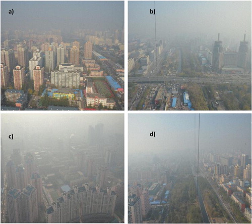
During the entire year of 2009, vertical flux and turbulence measurements were conducted using EC systems on a 325-m meteorological tower located in the northwest part of Beijing, China (39°58′N, 116°22′E) (Fig. 1). The elevation of the tower's base is 48.63 m above sea level. Within a 2-km radius around the measurement tower, the observational field is flat and consists mainly of many low- and high-rise residential housing units with average building heights of approximately 50 m in the southern direction and approximately 20 m in all other directions. The fractions covered by buildings (λ _b), vegetation (λ _v) and roads (λ _r) were 0.65, 0.23 and 0.12, respectively, as estimated based on digitised Google Maps. Within a 20-km radius of the tower, the mean building height is 18.3 m, and the λ _b, λ _v and λ _r were 0.65, 0.21 and 0.14, respectively (Miao et al., 2012). More detailed descriptions of the surface features surrounding the tower site, including the aerodynamic roughness length and zero-plane displacement, are found in Li et al. (2003) and Song and Wang (2012). In these references, the aerodynamic roughness length (), which varies with the wind direction and its spatial average, were 3.41 and 3.37 m determined from the horizontal wind profile under near-neutral conditions and from a roughness element morphology (Stull, 1988), respectively. The spatial zero-plane displacement length (z _d) was 26.4 m in the southern direction and approximately 13.5 m in other directions based on the wind profile data.

Fig. 1 Photographic views from the 325-m meteorological tower at a height of 140 m looking northward (a), eastward (b), southward (c) and westward (d). The photographs were taken on 16 November 2012. The weather condition was hazy.

2.2. Instruments

During the 2009 flux experiment, the instantaneous three-component velocities and temperatures were continuously measured using three-dimensional sonic anemometers (Model CSAT3, Campbell Scientific Inc., Logan, Utah, USA). The concentrations of CO₂ and water vapour were measured using open-path infrared gas analysers (Model LI-7500, LiCor Inc., Lincoln, NE, USA) fixed at three levels, 47, 140 and 280 m, above ground on a 325-m height, 2.7-m wide meteorological tower with a well-ventilated lattice structure. To reduce the effects of flow distortion from the tower, the instruments were mounted at the end of a 2.5-m boom and were pointed towards the south-east that was prevailing wind direction. The signals for the EC calculation at each level were sampled at a rate of 10 Hz and were recorded using dataloggers (model CR5000, Campbell Scientific Inc., Logan, Utah, USA) for postprocessing. In addition to the EC measurements, several meteorological variables were measured at multiple levels on the tower. Measurements of wind speed and direction, air temperature and relative humidity were collected at heights of 8, 15, 32, 47, 65, 100, 120, 140, 160, 180, 200, 240 and 280 m, whilst net radiation was recorded at 47, 140 and 280 m using radiometers (model CNR1, Kipp & Zonen, Delft, The Netherlands).

2.3. EC calculations

The turbulent fluxes of CO₂ (F _c), sensible heat (Q _H) and latent heat (Q _E) were measured using the configuration described above. The fluxes were obtained as the covariance (product) between the instantaneous deviation or fluctuations of vertical velocity () and their respective scalar () averaged over a time interval of 30 minutes1

where the overbar denotes a time average, N is the number of samples during the averaging time and the fluctuations are the differences between the instantaneous readings and their respective means. In our study, the average half-hourly turbulent fluxes were calculated and corrected using the Turbulence Knight 2 (TK2) software package from the University of Bayreuth, Germany (Mauder and Foken, 2004; Mauder et al., 2008). A more detailed description of the flux postprocessing is provided in Song and Wang (2012). In this application, the 30-minute flux calculations used despiked time series and a 2-D rotation correction; the 30-minute flux spectral density corrections used the transfer function methods of Moore (1986) and the Webb–Pearman–Leuning method proposed by Webb et al. (1980), respectively. The 30-minute flux quality assurance used a combination of the stationary test and the integral turbulence characteristics test proposed by Foken and Wichura (1996) and further developed by Foken et al. (2004). Table 1 shows that the whole-year flux data coverage of for CO₂, sensible heat and latent heat at three levels, 47, 140 and 280 m, ranged from 31 to 68% due to instrument malfunction, power failure, sensor calibration, precipitation and low-quality data. Gap filling was not attempted due to the complex nature of the CO₂ emissions above the urban surface (Vesala et al., 2008).

Table 1 The data coverage of turbulent fluxed measured at three levels 47, 140 and 280 m.

	Number of available half-hourly data points
Measurement heights (m)	CO2	Sensible heat	Latent heat
47	11 826 (68%, 24%*)	11 531 (65%, 26%*)	11 645 (66%, 26%*)
140	8759 (50%, 29%*)	6880 (39%, 44%*)	8196 (47%, 34%*)
280	8657 (49%, 42%*)	5494 (31%, 64%*)	8147 (46%, 46%*)

% in parentheses are the percentages of available data points.

*The fraction of data rejected by the stationary and the integral turbulence characteristics test applied.

3. Results and discussion

3.1. Meteorological conditions

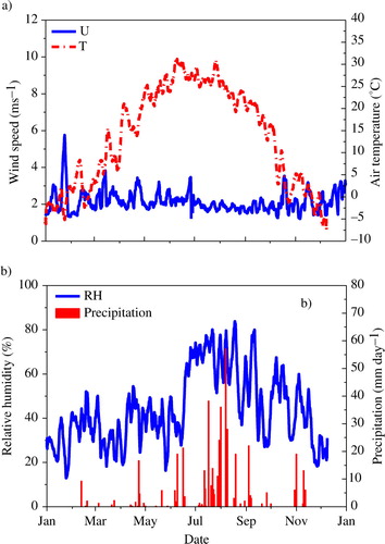
To provide a general characterisation of the meteorological conditions during the measurement period, meteorological factors including the 5-d running means of the air temperature, wind speed, relative humidity and daily precipitation at 32 m are presented (Fig. 2). The mean annual air temperature at 32 m was 13.7±11.7°C, which was warmer than the 20-yr climatic mean of 12.7±0.7°C. The extreme half-hour average air temperature during the study period ranged from −12.1°C on 23 February to 39.1°C on 18 June. Total precipitation measured on the roof of a two-storey office building near the tower was 472 mm in 2009, corresponding to approximately 87% of the 20-yr mean of 539 mm. The mean wind speed at 32 m was 2.2±1.3 m s⁻¹. The prevailing wind direction for this year was from the south-east with a 21% occurrence. Additionally, the mean relative humidity during the study period was 44.1±22.4%.

Fig. 2 (a) Five-day running means of the air temperature (°C) and wind speed (U, m s⁻¹), (b) precipitation (mm d⁻¹) and 5-d running means of the relative humidity (%) at a height of 32 m.

3.2. CO₂ flux

Positive CO₂ fluxes (F _c) were observed at three heights when data averaged over seasons (winter=DFJ, spring= MAM, summer=JJA and autumn=SON) as expected from an urban source area (Table 2). For F _c at three heights, winter time fluxes were higher than summer time fluxes that were consistent with observations at other urban sites (Soegaard and Møller-Jensen, 2003; Moriwaki and Kanda, 2004; Vesala et al., 2008; Matese et al., 2009; Helfter et al., 2011) and are also consistent with data from the previous year at the same study site (Song and Wang, 2012). The statistical distribution of winter time fluxes at three heights was not normally but skewed towards higher values (average mean was higher than average mean ), which indicated that fluxes in winter were more fluctuations. The difference of winter time fluxes among three heights was more significant in comparison with other seasons; of 1.32 mg m⁻² s⁻¹ at 47 m in winter time was 23 and 20% lower than that at 140 and 280 m, respectively. This could be attributed to few contributions of CO₂ sources such as heating to total fluxes measured at 47-m heights in view of sparse high chimneys for heating within the radius of 2 km around measurement tower that corresponded to the footprint of 47-m heights.

Table 2 Diurnally averaged half-hourly F _c (mg m⁻² s⁻¹), where h={1,2,3, … 48} for the half hours of the day and f _h as the set of flux data of all considered days for each h, is the average of all mean value, is the average of all median value, is the minimum and the maximum of the diurnal courses of the half hourly median .

Seasons	Measurement heights (m)			(LCT)
Winter	47	1.32	1.16	0.50 (0400)	1.84 (0800)
	140	1.70	1.50	0.79 (0400)	2.00 (1830)
	280	1.64	1.17	0.56 (0600)	2.10 (1730)
Spring	47	0.98	0.79	0.22 (0400)	1.24 (1900)
	140	0.76	0.67	0.35 (0300)	1.22 (1730)
	280	1.00	0.79	0.44 (0200)	1.29 (1730)
Summer	47	0.85	0.70	0.24 (0200)	1.25 (1900)
	140	0.82	0.73	0.30 (0200)	1.19 (1700)
	280	0.68	0.60	0.11 (1130)	1.19 (1700)
Autumn	47	0.89	0.72	0.22 (0200)	1.31 (1700)
	140	1.04	0.82	0.47 (0300)	1.28 (1730)
	280	0.94	0.66	0.33 (0330)	1.07 (1800)
Year	47	1.01	0.81	0.28 (0230)	1.24 (1930)
	140	1.07	0.85	0.51 (0230)	1.28 (1730)
	280	1.03	0.74	0.49 (0200)	1.20 (1730)

LCT in parentheses are the local time when the and were measured.

Two diurnal-pattern peaks in F _c were observed during the day in all seasons for three measurement heights, all maximum values occurred during the rush hours, around early morning for 47 m in winter and in late afternoon for 47, 140 and 280 m heights in other seasons. In view of the variation of traffic flow could be negligible during the entire year, the significant difference of between winter (ranged from 1.8 to 2.1 mg m⁻² s⁻¹) and other three seasons (ranged from 1.2 to 1.3 mg m⁻² s⁻¹) implied the contribution of CO₂ released by fossil fuel combustion for heating to total fluxes was important in winter. The all minimum values measured at three heights always occurred in the middle of the night when the anthropogenic activities were the lowest with the exception of that minimum value measured at 280 m in summer occurred around noon. The time of at 280 m in summer showed that the offsetting of emissions due to photosynthesis of the urban vegetation could affect the pattern of diurnal variation of F _c.

A wind-direction-dependent analysis of F _c at three heights can be derived from Fig. 3. A similar distribution of F _c for individual height with wind direction in summer and winter was observed. For 47-m measurement height that corresponded with about from 0.7 to 1 km footprint lengths under unstable and stable condition respectively, peak F _c linked with the wind directions aligned to the main roads (50 m to its east) and busy intersections (200 m to east-north) although these wind directions were not dominant during the entire year (Table 3), while fluxes from the direction of residential housing and vegetation showed lower fluxes. It was worth noting that the lowest F _c at 47 m was observed when fluxes came from the southern direction both in summer and winter seasons. This has to be attributed to a reduced vertical CO₂ transport due to the lid-effect of the overflowing air above the 50-m high buildings that was 200 m away from the measurement tower. A detailed lid-effect on F _c has been discussed by Lietzke and Vogt (2013), where lower F _c sampled at the top of the canyon (19 m) could be observed when wind direction was perpendicular to the street canyon. In contrast to the F _c at 47 m height, the lowest F _c at 140 m was observed for wind from east, and the highest F _c at 140 and 280 m corresponded with wind from north and west directions, respectively. The significant difference of magnitude of F _c from same wind direction among 47, 140, and 280 m heights demonstrated the effect of diverse urban surface covers contained by different footprints on measured F _c. Thus, the amalgamation of fluxes measured at different heights to improve data coverage for a better estimation of annual CO₂ emissions over urban landscape was problematic.

Fig. 3 The mean CO₂ flux measured at 47 m (left), 140 m (middle) and 280 m (right) and wind directions in winter (upper row) and in summer (lower row) by wind direction (45° intervals).

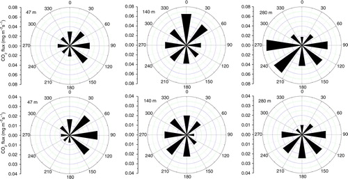
Table 3 The wind frequencies in different seasons by wind direction for 47-, 140- and 280-m measurement height

		Wind direction frequency (%)
Seasons	Wind sector (degrees)	47 m	140 m	280 m
Winter	0	9.95	16.25	13.37
	45	14.63	4.44	12.73
	90	13.97	9.98	12.38
	135	24.86	15.18	12.90
	180	8.20	12.85	14.78
	225	4.36	11.88	23.33
	270	12.11	9.75	5.62
	315	11.92	19.67	5.89
Summer	0	17.69	11.22	28.32
	45	11.29	4.18	16.25
	90	7.89	19.56	6.50
	135	13.11	26.99	4.44
	180	5.86	20.15	7.63
	225	4.01	4.28	15.09
	270	17.18	3.07	4.12
	315	22.97	10.55	17.64

It was difficult to quantify precisely the errors in CO₂ flux from urban area measured by EC technique (Velasco et al., 2005). Similar to the analysis taken by Velasco et al. (2005), we also assumed a random error of 20% and systematic error of 10% for each 30-minute mean flux to evaluate the uncertainty of seasonal CO₂ budget. When errors are random, errors in computed means diminish with increasing size of data set according to N ^−1/2, where N is the number of measurements. In contrast, systematic errors are not affected by increasing data size, because they simply add in linear manner. By adding the random errors and systematic errors in quadrature (Moncrieff et al., 1996), Table 4 showed the total uncertainty of CO₂ budget varied from ±1.54 to ±0.71 kg m⁻² season⁻¹ (i.e. 280 m) with seasons, which was 11.6 and 13.2% of total fluxes. In general, the uncertainty at three measurement heights was all limited within 13.5%.

Table 4 Seasonal CO₂ fluxes budget estimated at 47-, 140- and 280-m measurement height

	CO2 flux (kg m^−2 season^−1)
Seasons	47 m	140 m	280
Winter	10.64 (±1.18)	13.61 (±1.51)	13.34 (±1.54)
Spring	7.95 (±0.93)	6.10 (±0.72)	8.03 (±0.96)
Summer	6.82 (±0.84)	6.58 (±0.79)	5.40 (±0.71)
Autumn	7.25 (±0.88)	8.38 (±0.97)	7.34 (±0.90)

The values in parentheses were uncertainty of fluxes.

A mean annual CO₂ flux estimate at 47, 140, and 280 m height of 32.6, 34.6 and 34.2 kg m⁻² yr⁻¹, respectively, was calculated for the year 2009. It is somewhat surprising that the difference in annual CO₂ flux estimated among three heights was less than 5% in view of diverse urban surface covers contained by footprints corresponded to three different heights. This CO₂ flux (e.g. 47 m) is considerably higher than in most urban and suburban sites with the exception of the centre London study (35.5 kg CO₂ m⁻² yr⁻¹) (Helfter et al., 2011). The annual CO₂ emissions from urban areas of Copenhagen (Soegaard and Møller-Jensen, 2003), residential areas of Tokyo (Moriwaki and Kanda, 2004), residential areas of Melbourne (Coutts et al., 2007), the urban centre area of Lodz (Pawlak et al., 2011) and suburban areas of Montreal (Bergeron and Strachan, 2011) were 59, 64, 71, 65 and 82% lower, respectively, than that observed at 47 m at our site. Although the CO₂ flux of 20.6 kg m⁻² yr⁻¹ measured at a single height of 47 m in 2008 (Song and Wang, 2012) was considered to reflect the reduction of emissions to the atmosphere during the Olympic Games, the estimate of 32.6 kg m⁻² yr⁻¹ obtained using data measured in 2009 at 47-m heights, appeared to be inexplicably higher than in 2008. Using a linear correlation between the mean air temperature and the mean monthly CO₂ flux measured in 2008 (Song and Wang, 2012), we predicted that the mean annual CO₂ flux in 2009 was only approximately 22 kg m⁻² yr⁻¹; this prediction indicates that the significant inter-annual CO₂ flux difference is only partly explained by the air temperature variability that corresponded to fossil fuel combustion for heating in the cold seasons during those 2 yr. The variability of other CO₂ sources between these years should be incorporated to better interpret the inter-annual difference. For example, using an inventory method for vehicle fuel consumption, as reported by Song and Wang (2012), the observed increase of 0.52 million vehicles over this period (3.5 and 4.02 million vehicles in Beijing in 2008 and 2009, respectively) resulted in an annual CO₂ flux increase of 2.8 kg m⁻² yr⁻¹ during 2009. Additionally, the reopening of factories after the Olympic Games may also have contributed to the higher annual CO₂ flux in 2009 (Liu et al., 2012), although this contribution to the total CO₂ flux was difficult to quantify.

3.3. Energy balance fluxes

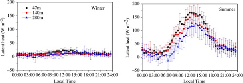
The diurnal courses of the average seasonal sensible heat (Q _H), latent heat flux (Q _E) at three heights are presented in Figs. 4 and 5. The daytime maximum of Q _H was 105 W m⁻² at the 47 m height in summer and approximately 102 W m⁻² at the same height in winter (Fig. 4). This similarity of the Q _H daytime peak between summer and winter could be attributed to the clear distinction of climate between dry (winter) and wet (summer) seasons in Beijing (Liu et al., 2012). A decrease of the daytime Q _H with increasing height was apparent in winter and was attributed to the fact that the lowest level was directly and strongly influenced by the nearby buildings that acted as heat sources and the absence of an evaporating medium in winter. Negative values of Q _H (approximately from −3 to −10 W m⁻²) measured at all three heights, occurred during the majority of summer nights (≥7 hours), indicated a slightly stable stratification associated with the nocturnal urban boundary in summer. During the winter nights, the Q _H at 47 and 140 m were both positive (up to 10 W m⁻²), while Q _H at 280 m approached zero, indicating that the lower region of the urban boundary layer remained slightly unstable, while the stratification was more neutral above this transition layer. Positive values of Q _H occurred in the lower parts of the boundary layer in winter, possibly because of higher anthropogenic heat input during these periods. In summer, our results showed lower peak Q _H values compared with those from other high-latitude urban sites. In Helsinki, Vesala et al. (2008) reported a Q _H of 300 W m⁻² during the summer daytime over urban and road sectors. Nordbo et al. (2012) reported that Q _H could reach 560 W m⁻² in the summer daytime over the north-eastern areas of downtown Helsinki. Our results could be considered comparable to those obtained for lower latitude urban flux sites; for example, in the city centre of Mexico City, Q _H remained positive with a peak value of approximately 130 W m⁻² through the dry season (Oke et al., 1999). Martin et al. (2009) observed peak wintertime and summertime Q _H values ranging from 50 to 160 W m⁻² in Edinburgh and from 160 to 210 W m⁻² in Manchester, UK, respectively, between 1999 and 2006, but also noted differences when average weekday values were compared to weekend values. Diurnal cycles in Gothenburg, Sweden, were found to be significantly smaller in range. The average diurnal Q _E values (Fig. 5) were consistently positive during the entire measurement period. A diurnal-pattern peak in Q _E was observed during the day in the summer season. The daytime Q _E maximum was 167 W m⁻² at the 47-m height in the summer but only 23 W m⁻² at the same height in the winter. Grimmond and Oke (2002) analysed Q _E data from 10 urban sites and found that the daily peak values ranged from 20 to 250 W m⁻². In summer, the seasonal mean hourly Q _E measured in urban areas of Helsinki (Vesala et al., 2008; Nordbo et al., 2012), Basel (Vogt et al., 2006) and London (Helfter et al., 2011) could approach 150, 95, 100 and 60 W m⁻², respectively. In a suburban area of Tokyo, the mean hourly Q _E was approximately 200 W m⁻² for sunny summer days (Moriwaki and Kanda, 2004). The Bowen ratio (Q _H/Q _E) varied with the season. The wintertime values were the greatest overall because the least precipitation and evapotranspiration also occurred in winter, whereas the summertime values were the smallest in terms of higher evaporation and transpiration in summer. The peak daytime ratio value was approximately 8 in winter and less than 1 in the summer. Using the same data, Miao et al. (2012) observed that the Bowen ratio varied with the wind direction and measurement height.

Fig. 4 The diurnal course of the average seasonal sensible heat in the winter and summer measured at three heights (47, 140 and 280 m). The vertical line indicates the standard deviation.

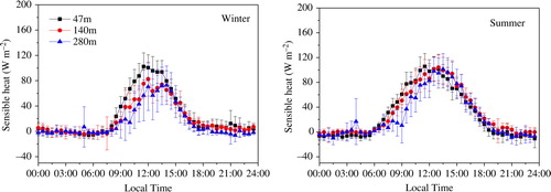
Fig. 5 The diurnal course of the average seasonal latent heat in the winter and summer measured at three heights (47, 140 and 280 m). The vertical error bars indicate the standard deviation.

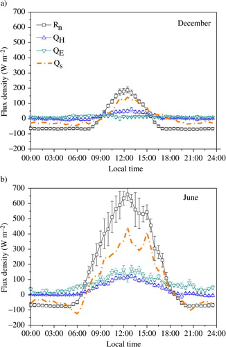
As shown in Figs. 4 and 5, the diurnal courses of the different surface energy balance components were similar at each of the three heights. The energy fluxes measured at 140 m were used to analyse the surface energy balance (Fig. 6). The direct observation of the storage heat flux is difficult in urban areas due to the complex urban surface structure and the diversity of material types that comprise the urban interface (Moriwaki and Kanda, 2004). Therefore, the storage heat flux was determined as a residual from the direct observations of the net radiation (Rn), sensible heat (Q _H) and latent heat flux (Q _E)2

Fig. 6 The diurnal course of the average monthly energy fluxes in (a) December and (b) June at a 140-m height. The vertical line indicates the standard deviation.

Here, the heat storage in the air between the surface and the measurement height Q _A was determined from the air volumetric heat capacity and the vertical temperature profiles measured between the surface and the measurement height. Q _A varied greatly in a diurnal course during the all seasons, for example, it ranged from −23 W m⁻² in the mid-night to 65 W m⁻² in the noon in winter (figure not shown). The 65 W m⁻² of daily maximum estimated at our site indicated that Q _A was comparable in magnitude to the turbulent heat fluxes, and therefore could not be neglected in the discussion of energy balance fluxes on a half-hourly and hourly basis. However, mean daily Q _A during the year of 2009 was −0.14 W m⁻², and the yearly sum was only −4.42×10⁻³ GJ yr⁻¹m⁻², which indicated that Q _A integrated for a day or for longer time scales was negligible when we compared it with the other components of energy balance fluxes.

Errors associated with turbulent heat fluxes measured in urban areas can be approximately 9–16% of the measured fluxes (Nordbo et al., 2012), and the cumulative errors of the storage heat flux from these measurement uncertainties may therefore be significant. Thus, the heat storage result presented here should be treated with caution. The heat storage (Q _S) derived from the residual of the energy balance ranged from −145 to 404 W m⁻² in the summer months and from −95 to 90 W m⁻² in the winter months. The nightly averages for both summer and winter data were consistently negative, indicating the release of heat from storage (Fig. 6). The daily average of Q _S are positive in summer month, suggesting that more heat was stored than released from anthropogenic sources, whereas values in winter months are found to be negative. The residual term of the energy balance equation Rn−(Q _H+Q _E+Q _A) showed small values in the yearly total. This suggested a missing energy source of the order of 0.78±0.26 GJ yr⁻¹m⁻² for the Beijing urban heat budget. Here, the uncertainty of annual missing energy was estimated by assuming a systematic error of 10% for each 30-minute mean turbulent heat fluxes and neglecting random error for heat fluxes in view of the fact that random errors would be minor with dataset size increasing to a year. The annual total of Qs has to be zero by definition as the city cannot be expected to cool down or heat up (Christen and Vogt, 2004), and hence the missing source was attributed to the anthropogenic heat flux density Q _F. Here, the assumed constant anthropogenic emission suggested a Q _F of approximately 25±8.6 W m⁻² in the annual average.

3.4. Turbulence characteristics

The intense turbulence created over rough surface can be expressed through the drag coefficient, C _D, which is required for many practical purposes, such as relating the momentum flux to the mean wind profile, and parameterisation of the surface stress in numerical models (Roth, 2000). The form of drag coefficient is3 where u* is the friction velocity and U is the mean wind speed, is frequently used to describe the effect of surface roughness on the turbulence and wind fields. Note that for a given surface, C _D decreases with height when the atmosphere is stable, that is4

where z _S is the measurement height, z _d is the zero-plane displacement plane and L (the Obukhov length) is neutral (defined as ). Figure 7 shows the variation of C _D ^0.5 with non-dimensional heights ( and Z _S /Z _H , where and Z _H , respectively, is the average canopy height) under neutral conditions. The data observed at higher levels are comparable to the log law wind profile [eq. (5)] and the line [eq. (6)] predicted by Roth (2000) are similar to data observed in other urban sites.5 6

Fig. 7 Variation of the drag coefficient for neutral conditions with non-dimensional height (a) and (b) z _S/z _H . The line on the left is eq. (5), and the line on the right is eq. (6). The squares are data from this study, and the asterisks are data reported by Roth (2000) and Grimmond et al. (2004).

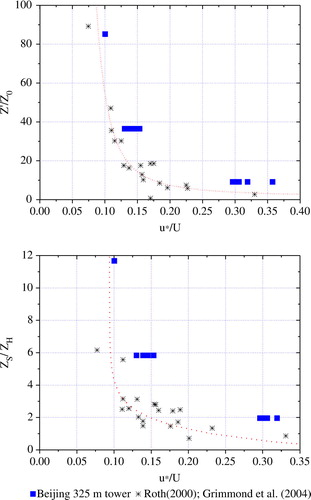
Similar to the results reported by Roth (2000), the data observed at lower levels showed a broad scatter and bias with respect to the theoretical and empirical line. The values of C _D observed at the non-dimensional heights () of 9, 36 and 85 in neutral stratification were 0.09, 0.02 and 0.01, respectively, which are comparable with those of 0.01~0.03 observed at 150~280 m rooftops in New York (Hanna and Zhou, 2007) and higher than that of 0.008 observed on a 190-m tower in London (Wood et al., 2010).

It is important to specify the standard deviations of the wind velocities () in many dispersion applications (Grimmond et al., 2004). The form of normalised standard deviations of the wind velocity components is7

Here, A _i for longitudinal (u), lateral (v) and vertical (w) wind velocities were analysed for neutral conditions. The values of A _u at 47, 140 and 280 m ranged from 1.8 to 2.0 with a mean of 1.91. The values of A _v observed at these three heights ranged from 1.5 to 1.7 with a mean of 1.6; A _w showed a large variability and ranged from 0.77 to 1.1 with a mean of 1.0. In all cases, these values were smaller than those reported in previous studies, for example, (i) 2.23, 1.81 and 1.25 for A _u , A _v and A _w , respectively, suggested by Roth (2000) for Z _S /Z _H >2.5; (ii) 2.3, 1.85 and 1.35 for A _u , A _v and A _w , respectively, observed on a 190-m tower in London (Wood et al., 2010) and (iii) values observed in other cities, which were summarised by Wood et al. (2010, see Table 1). The REPARTEE study by Harrison et al. (2012) conducted over the city of London also showed good agreement between turbulence observations and the model prediction by Roth (2000).

The turbulence production rate and its intensity are defined as follows:8

Figure 8 shows that the turbulence intensity varied with the non-dimensional heights for neutral conditions. The line is based on the theory equation [Roth, 2000, eq. (8)]9 and Roth's empirical equations [Roth, 2000, eq. (9)]10 11 12

Fig. 8 The variation of (top), (middle) and (bottom) for neutral conditions with non-dimensional height (left) and z/z _H (right). The line on the left is from Roth (2000) based on theory, that is, his eq. (8), and the line on the right is from his empirical equation (9).

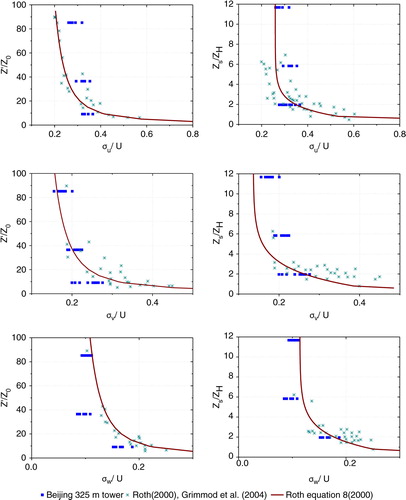
The data observed at the three heights were comparable to those observed in other urban sites and could be described by both lines. Similar to the results reported by Roth (2000), the turbulence intensities of I _u and I _v showed more variation around the theoretical [eq. (9)] and empirical lines [eqs. (10) and (11)], and the values tended to be smaller compared with equations at lower levels. Whereas, the I _w measured at our site did not follow the theoretical [eq. (9)] and empirical lines [eq. (12)] well and their values at middle level was smaller than that at upper levels. When turbulence intensities were plotted against the stability (Fig. 9), a considerable scatter around the Monin–Obukhov similarity predictions was evident for I _u , and a clear increasing trend in the ratio from the unstable to the neutral side was not evident. In contrast to I _u , the data for I _v and I _w were similar to the Monin–Obukhov similarity predictions and showed an increasing trend with increasing instability. The variation of I _i under stable conditions has received relatively less consideration in previous studies. Roth (2000) and Grimmond et al. (2004) summarised and analysed the variation of I _i in the stability regime ranging from −2 to 0.5. For our study, there were no significant decreases in I _v and I _w with increasing stability when

Fig. 9 Variation of the turbulence intensity with stability. The data from this study are the means for each 0.5 interval of stability. Dot-dash lines are from Roth [2000, eq. (10)].

4. Conclusions

The multiple height EC measurements over urban areas of Beijing conducted here can substantially enrich the worldwide CO₂ and energy balance fluxes database to the nascent tall tower flux measurements in urban area. The fluxes of sensible and latent heat showed substantial diurnal and seasonal variations. Although the fluxes of sensible and latent heat at 47, 140 and 280 m exhibited similar diurnal patterns, differences in the magnitudes of these fluxes between the levels were significant in certain seasons. The annual CO₂ budget in 2009 estimated by the combination of data measured at the 47-m levels was 32.6 kg m⁻² yr⁻¹, which was not only considerably higher than that for most other reported cities but was also higher than that for the previous year at the same study site. An increase in road traffic is thought to be an obvious contributor to the increase of annual CO₂ emissions in 2009. It is evident that the CO₂ emissions from Beijing are at a high level and energy consumption of related to CO₂ emissions is accelerated, which implies that the mitigation of CO₂ in areas undergoing rapid urbanisation is a urgent issue.

The turbulent data measured at three levels allowed for a comparison with the urban area turbulent vertical profiles summarised by previous studies. The drag coefficient (C _D) values observed at the non-dimensional heights () of 9, 36 and 85 in neutral stratification were 0.09, 0.02 and 0.01, respectively, which were comparable to previous results for urban areas (e.g., Hanna and Zhou, 2007; Wood et al., 2010). The variation of the turbulence intensity with non-dimensional heights for neutral conditions supported the empirical functions proposed by Roth (2000).

5. Acknowledgments

This work was supported by the Program of 100 Distinguished Young Scientist of the Chinese Academy of Sciences (No.: 7-102151), the National Natural Science Foundation of China (No.: 41275139) and the CAS Strategic Priority Research Program Grant (XDA05100100). The authors thank Aiguo Li and Jingjing Jia for their technical assistance with installing and maintaining the measurement equipment. The comments of the anonymous reviewers have helped substantially to improve this article.

References

- Baldocchi D . Assessing the eddy covariance technique for evaluating carbon dioxide rates of ecosystems: past, present and future. Glob. Change Biol. 2003; 9: 479–492.
- Baldocchi D , Falqe E , Gu L. H , Olson R , Hollinger D , co-authors . FLUXNET: a new tool to study the temporal and spatial variability of ecosystem-scale carbon dioxide, water vapour, and energy flux densities. Bull. Am. Meteorol. Soc. 2001; 82: 2415–2434.
- Bergeron O , Strachan I . CO2 sources and sinks in urban and suburban areas of a northern mid-latitude city. Atmos. Environ. 2011; 45: 1564–1573.
- Burri S , Frey C , Parlow E , Vogt R . CO2 fluxes and concentrations over an urban surface in Cairo/Egypt. The seventh International Conference on Urban Climate. 2009. Yokohama, Japan, 29 June–3 July.
- Christen A , Vogt R . Energy and radiation balance of a central European city. Int. J. Climatol. 2004; 24: 1395–1421.
- Coutts A. M , Beringer J , Tapper N. J . Characteristics influencing the variability of urban CO2 fluxes in Melbourne, Australia. Atmos. Environ. 2007; 41: 51–62.
- Crawford B , Grimmond C , Christen A . Five years of carbon dioxide fluxes measurements in a highly vegetated suburban area. Atmos. Environ. 2011; 45: 896–905.
- Dorsey J , Nemitz E. G , Gallagher M. W , Theobold M , Fowler D . Tower based measurements of micrometeorological exchange parameters and heat fluxes above a city. Nucl. Atmos. Aerosols. 2000; 534: 646–649.
- Foken T , Gockede M , Mauder M , Mahrt L , Amiro B. D , co-authors . Lee X . Post-field data quality control. Handbook of Micrometeorology: A Guide for Surface Flux Measurements. 2004; Dordrecht: Kluwer. 181–208.
- Foken T , Wichura B . Tools for quality assessment of surface-based flux measurements. Agr. Forest Meteorol. 1996; 78: 83–105.
- Frey C. M , Parlow E , Vogt R , Harhash M , Wahab M. M. A . Flux measurement in Cario. Part 1: in situ measurement and their applicability for comparison with satellite data. Int. J. Climatol. 2011; 31: 218–231.
- Grimmond C. S. B , Salmond J. A , Oke T. R , Offerle B , Lemonsu A . Flux and turbulence measurements at a densely built-up site in Marseille: heat, mass (water and carbon dioxide), and momentum. J. Geophys. Res. 2004; 109: 24101–24120.
- Grimmond C. S. B , Oke T. R . Turbulent heat fluxes in urban areas: Observations and a Local-Scale Urban Meteorological Parameterization Scheme (LUMPS). J. Appl. Meteorol. 2002; 41: 792–810.
- Hanna S , Zhou Y . Results of analysis of sonic anemometer observations at street level and rooftop in Manhattan. 6th International Conference on Urban Air Quality.
- Harrison R. M , Dall'Osto M . Atmospheric chemistry and physics in the atmosphere of a developed megacity (London): an overview of the REPARTEE experiment and its conclusions. Atmos. Chem. Phys. 12
- Helfter C , Famulari D , Phillips G , Barlow J , Wood C , co-authors . Controls of carbon dioxide concentrations and fluxes above central London. Atmos. Chem. Phys. 2011; 11: 1913–1928.
- Li Q , Liu H. Z , Hu F , Hong Z. X , Li A. G . The determination of aero dynamical parameters over urban land surface. Clim. Environ. Res. 2003; 8: 444–450. (in Chinese with English abstract).
- Lietzke B , Vogt R . Variability of CO2 concentrations and fluxes in and above and urban street canyon. Atmos. Environ. 2013; 74: 60–72.
- Liu H. Z , Feng J. W , Järvi L , Vesala T . Four year (2006–2009) eddy covariance measurements of CO2 flux over an urban area in Beijing. Atmos. Chem. Phys. 2012; 12: 7881–7892.
- Martin C. L , Longley I. D , Dorsey J , Thomas R. M , Gallagher M. W , co-authors . Ultrafine particle fluxes above four major European cities. Atmos. Environ. 2009; 43: 4714–4721.
- Matese A , Gioli B , Vaccari F. P , Zaldei A , Miglietta F . Carbon dioxide emissions of the city centre of Firenze, Italy: measurement, evaluation, and source partitioning. J. Appl. Meteorol. Climatol. 2009; 48: 1940–1947.
- Mauder M , Foken T . Documentation and Instruction Manual of the Eddy Covariance Software Package TK2. Work report. 2004; 26: 45. University of Bayreuth, Department of Micrometeorology Internet.
- Mauder M , Foken T , Clement R , Elbers J. A , Eugster W , co-authors . Quality control of CarboEurope flux data – Part 2: inter-comparison of eddy-covariance software. Biogeosciences. 2008; 5: 451–462.
- Miao S. G , Dou J. X , Chen F , Li J , Li A. G . Analysis of observations on the urban surface energy balance in Beijing. Sci. China Earth. Sci. 2012; 55: 1881–1890.
- Moncrieff J. B , Mahli Y , Leuning R . The propagation of errors in long term measurements of land atmosphere fluxes of carbon and water. Glob. Change Biol. 1996; 2: 231–240.
- Moore C. J . Frequency response correction for eddy correction systems. Boundary Layer Meteorol. 1986; 37: 17–30.
- Moriwaki R , Kanda M . Seasonal and diurnal fluxes of radiation, heat, water vapor, and carbon dioxide over a suburban area. J. Appl. Meteorol. 2004; 43: 1700–1710.
- Nemitz E , Hargreaves K. J , McDonald A. G , Dorsey J. R , Fowler D . Meteorological measurements of the urban heat budget and CO2 emissions on a city scale. Environ. Sci. Technol. 2002; 36: 3139–3146.
- Nordbo A , Järvi L , Vesala T . Revised eddy covariance flux calculation methodologies- effect on urban energy balance. Tellus B. 2012; 64: 18184.
- Offerle B , Grimmond C. S. B , Fortuniak K , Klysik K , Oke T. R . Temporal variation in heat fluxes over a central European city centre. Theor. Appl. Climatol. 2006; 84: 103–115.
- Oke T. R , Spronken-Smith R. A , Jáuregui E , Grimmond C. S. B . The energy balance of central Mexico City during the dry season. Atmos. Environ. 1999; 33: 3919–3930.
- Pawlak W , Fortuniak K , Siedlecki M . Carbon dioxide flux in the centre of LŁódź, Poland-analysis of a 2-year eddy covariance measurement data set. Int. J. Climatol. 2011; 31: 232–243.
- Roth M . Review of atmospheric turbulence over cities. Q. J. R. Meteorol. Soc. 2000; 126: 941–990.
- Soegaard H , Møller-Jensen L . Towards a spatial CO2 budget of a metropolitan region based on textural image classification and flux measurements. Rem. Sens. Environ. 2003; 87: 283–294.
- Song T , Wang Y. S . Carbon dioxide fluxes from an urban area in Beijing. Atmos. Res. 2012; 106: 139–149.
- Stull R . An Introduction to Boundary Layer Meteorology (Chinese version) . 1988; China Meteorological Press, Beijing. 401–405.
- Velasco E , Pressley S , Allwine E , Westberg H , Lamb B . Measurements of CO2 fluxes from the Mexico City urban landscape. Atmos. Environ. 2005; 39: 7433–7446.
- Vesala T , Järvi L , Launiaine S , Sogachev A , Rannik Ü , co-authors . Surface–atmosphere interaction over complex urban terrain in Helsinki, Finland. Tellus B. 2008; 60: 188–199.
- Vogt R , Christan A , Rotach M. W , Roth M , Satyanarayana A. N. V . Temporal dynamics of CO2 fluxes and profiles over a central European city. Theor. Appl. Climatol. 2006; 84: 117–126.
- Webb E. K , Pearman G. I , Leuning R . Correction of flux measurements for density effects due to heat and water vapour transfer. Q. J. R. Meteorol. Soc. 1980; 106: 85–100.
- Wood C. R , Lacser A , Barlow J. F , Padhra A , Belcher S. E , co-authors . Turbulent flow at 190 m heights above London during 2006–2008: a climatology and the applicability of similarity theory. Boundary Layer Meteorol. 2010; 137: 77–96.