Allowable carbon emissions for medium-to-high mitigation scenarios

Abstract

Using an ensemble of simulations with an intermediate complexity climate model and in a probabilistic framework, we estimate future ranges of carbon dioxide (CO₂) emissions in order to follow three medium-high mitigation concentration pathways: RCP2.6, RCP4.5 and SCP4.5 to 2.6. Uncertainty is first estimated by allowing modelled equilibrium climate sensitivity, aerosol forcing and intrinsic physical and biogeochemical processes to vary within widely accepted ranges. Results are then constrained by comparison against contemporary measurements. For both constrained and unconstrained projections, our calculated allowable emissions are close to the standard (harmonised) emission scenarios associated with these pathways. For RCP4.5, which is the most moderate scenario considered in terms of required emission abatement, then after year 2100 very low net emissions are needed to maintain prescribed year 2100 CO₂ concentrations. As expected, RCP2.6 and SCP4.5 to 2.6 require more strict emission reductions. The implication of this is that direct sequestration of carbon dioxide is likely to be required for RCP4.5 or higher mitigation scenarios, to offset any minimum emissions for society to function (the ‘emissions floor’). Despite large uncertainties in the physical and biogeochemical processes, constraints from model-observational comparisons support a high degree of confidence in predicting the allowable emissions consistent with a particular concentration pathway. In contrast the uncertainty in the resulting temperature range remains large. For many parameter sets, and especially for RCP2.6, the land will turn into a carbon source within the 21st century, but the ocean will remain as a carbon sink. For land carbon storage and our modelling framework, major reductions are seen in northern high latitudes and the Amazon basin even after atmospheric CO₂ is stabilised, while for ocean carbon uptake, the tropical ocean regions will be a source to the atmosphere, although uncertainties on this are large. The parameters which most significantly affect the allowable emissions are aerosols and climate sensitivity, but some carbon-cycle related parameters (e.g. maximum photosynthetic rate and respiration's temperature dependency of vegetation) also have significant effects. Parameter values are constrained by observation, and we found that the CO₂ emission data had a significant effect in constraining climate sensitivity and the magnitude of aerosol radiative forcing.

• climate-carbon cycle system
• earth system model of intermediate complexity
• parametric uncertainty
• observational constraints
• allowable emissions
• Representative Concentration Pathways

1. Introduction

Following the protocol of the Coupled Model Intercomparison Project Phase 5 (CMIP5), climate research centres are running high resolution General Circulation Models (GCMs), some of which contain carbon cycle components and are called Earth System Models (ESMs), forced by Representative Concentration Pathway (RCP) scenarios (Meinshausen et al., 2011b). These prescribe atmospheric gas concentrations. Studies now report allowable emissions for single simulations by each ESM forced with such RCPs (Arora et al., 2011; Hajima et al., 2012), and Jones et al. (2013) summarise these allowable emissions for CMIP5 models. Jones et al. (2013) found that future projections for RCP2.6 and RCP4.5 are consistent with Integrated Assessment Model (IAM) estimates (the harmonised emission scenario), whilst for high end scenarios (RCP6.0 and 8.5) ESMs simulate smaller allowable (‘compatible’) emissions than the IAMs.

RCPs are concentration pathways and, therefore, for those scenarios we can calculate both allowable emission and temperature rise for each model. Allowable emissions are the anthropogenic emissions that corresponds to a prescribed atmospheric CO₂ pathway (i.e. what humans are ‘allowed’ to emit to achieve that pathway) and is equivalent to the sum of the changes in air-, ocean- and land-borne carbon for the given concentration pathway. As expected, these are model-dependent and can vary from the MAGICC ‘harmonised’ values (Meinshausen et al., 2011b). Such variation can depend on, for instance, alternative implicit climate sensitivities, varying depictions of the global carbon cycle and carbon-cycle feedbacks in response to changing CO₂ concentration or climate (Gregory et al., 2009). The CMIP5 integrations exhibit large differences, and thus, uncertainties in physical and carbon cycle process representation (Arora et al., 2013). An understanding of how such uncertainty affects allowable emissions, and also temperature responses to the RCPs, is important for future planning. However given the massive computational requirement and long run times, creating ensembles of full ESMs remains difficult. Hence the limited number of CMIP5 integrations means that we need to rely additionally on other tools to assess the implication of process uncertainty on allowable future emissions. Many researchers (e.g. Lenton, 2000; Meinshausen et al., 2011a, c) have made parameter perturbation experiments with simpler global ‘box’ models, which provide general information on climate evolution through use of globally effective parameters. Whilst such studies can be very informative, they may not inform on the intricate background mechanisms behind the change in global mean or globally integrated values. Our solution to this problem is to utilise a modelling structure that falls between the two extremes. We use a Loosely Coupled Model (LCM, Tachiiri et al., 2010). This model uses predictions from a fast Earth system Model of Intermediate Complexity (EMIC) to scale pre-computed climatic fields from an existing full GCM, thus producing a large ensemble of three-dimensional results. However each ensemble member, which has a different parameterisation, requires only a fraction of the computational cost of a full ESM simulation.

Here we use ensembles from the LCM to define the magnitude and assess uncertainty in future allowable carbon emissions for particular RCPs. These are the ‘benchmark’ concentration scenarios that have been developed (Moss et al., 2010) for use by state-of-the-art climate models in preparation for the forthcoming fifth IPCC Assessment Report. We focus on the medium (Taylor et al., 2009) to high mitigation (or low to medium-low emission) scenarios, RCPs 2.6 and 4.5, including extensions to year 2300. In addition, we also analyse SCP4.5 to 2.6, a supplementary extension from RCP4.5. RCP4.5 assumes additional atmospheric radiative forcing through anthropogenic activities to increase to around 4.5 W/m² by year 2120 and remains constant thereafter, and of which most of this altered radiative forcing is due to changed concentrations of atmospheric CO₂. RCP2.6 (sometimes called RCP-3PD) assumes additional atmospheric radiative forcing of 3 W/m² in the peak period but then declines to 2.6 W/m² in 2100. SCP4.5 to 2.6 follows RCP4.5 until 2100 and then starts to approach RCP2.6 to join that in 2250. For each RCP and SCP scenario a baseline ‘harmonised’ emission scenario is available, produced by a single model (MAGICC, Meinshausen et al., 2011a, b, c) with a climate sensitivity of 3 K.

In this study, we present a consolidated framework that captures uncertainty bounds in identifiable model parameters, and that are both consistent with the scientific consensus presented by the last IPCC report and also individually, based on expert opinion for each parameter. Constraints, subject to caveats below, are provided using a comprehensive set of contemporary and recent-past observations. It is these bounds and constraints that enable the building of a probabilistic framework to assess allowable emissions and temperature rise with medium-to-high mitigation scenarios. The recent paper by Bodman et al. (2013) represents a major step forward in understanding the implications of the global carbon cycle uncertainty on future temperature rise, with a use of simple MAGICC model and global temperature and CO₂ observation. Here we present the next logical step, constraining the climate-carbon cycle model with a step-change increase in complexity. Comparing our ensemble to a much wider use of observational comparisons allows us to weight down less credible model projections.

We present the model, scenario, parameter sets perturbed and observation data we use in Section 2. In Section 3 we show output of our ensemble members associated with medium-to-high mitigation emission scenarios, mainly in terms of allowable emission. The discussion, including temperature response and also spatial distribution of the land/ocean carbon storage, is in Section 4. The conclusions follow in Section 5. Some methodological description is also presented in an Appendix.

2. Methods

2.1. Model and experiments

The Japan Uncertainty Modelling Project – Loosely Coupled Model (JUMP-LCM, Tachiiri et al., 2010) loosely couples MIROC-lite (Oka et al., 2011) with the land surface model Sim-CYCLE (Ito and Oikawa, 2002). MIROC-lite is a simplified atmosphere–ocean coupled model including a marine ecosystem component, and Sim-CYCLE is driven by an archive of meteorological outputs from a full GCM: MIROC3.2 medium resolution version (K-1 model developers, 2004). Together these mimic the full ESM, MIROC3-ESM (called FRCGC in C4MIP, Yoshikawa et al., 2008). JUMP-LCM is computationally efficient, and it therefore allows massive ensembles to be made across parameter ranges. Such parameter ranges can be associated with a probability distribution, based on expert opinion. Then in a further comparison to contemporary measurements, this enables each ensemble member to be prescribed an overall weighting. When all members are combined, this gives a full probability distribution for allowable emissions, and also for predicted future temperature ranges. For each simulation and corresponding parameters, a long spin-up period to pre-industrial conditions is performed to ensure a steady state is achieved (3000 yr for MIROC-lite component and 2000 yr for Sim-CYCLE component). As the evolution of the terrestrial and marine ecosystem carbon pools provide a strong control on allowable anthropogenic emissions, for the land surface we adopt a sophisticated model in full, Sim-CYCLE.

To retain low computational expense, the land surface component is also loosely coupled, and only passes back to MIROC-lite yearly changes in carbon stocks. This lack of full coupling does mean that other more regional types of feedbacks, including effects of changed surface albedo and evaporation due to modelled altered land surface conditions, are not presently captured in this system. The influence of land use change on the carbon cycle is also treated relatively simply. Sim-CYCLE does not have an explicit pasture functional type, so we treat this as the same as cropland, tuning its parameterisation so that the resultant net land use emission is consistent with estimated values (Fig. 1 of Houghton et al., 2012). Albedo change due to land surface change is included in the radiative forcing data in the RCP scenarios.

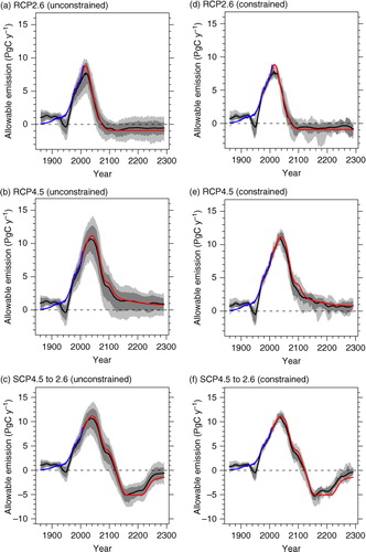
Fig. 1 Time series of allowable annual fossil fuel emissions for period 1850–2300.RCP2.6 (a), RCP4.5 (b) and SCP4.5 to 2.6 (c). The black curve is the ensemble mean, and the dark and light grey shades correspond to 68 (16–84 percentile) and 90 (5–95 percentile)% ranges respectively. The blue curve is the historical estimates of emissions (Carbon Dioxide Information Analysis Center: http://cdiac.ornl.gov/ftp/ndp030/global.1751_2009.ems). The red curves are harmonised RCP emissions (derived from MAGICC, documented in Meinshausen et al., 2011a). (d)–(f) are same as (a)–(c) but now for our constrained set of simulations using the eight observed datasets in Table 2.

Our ensemble contained 512 simulations. The parameters selected are generated using a Latin hypercube, based on the parameter bounds of Table 1, and so that there is minimised correlation between the parameters. Initially all parameter perturbations (Table 1) are assumed to have probabilities from a uniform distribution. However, a uniform distribution in climate sensitivity is known not to be realistic (Annan and Hargreaves, 2009). Hence we adopt probability distributions for climate sensitivity and aerosol-derived radiative forcing based on the fourth IPCC Assessment Report (AR4) (Forster et al., 2007; Hegerl et al., 2007). Thus we use non-flat priors for these parameters. It should be noted that other radiative forcings than aerosol, e.g. GHGs and land-cover change albedo, are not varied in this study. Detail of the priors for climate sensitivity and aerosol forcing are given in Appendix A; how we determined the parameter perturbation ranges are in Appendix B and a description of these parameters is given in Appendix C.

Table 1  Parameters perturbed in this study and the ranges considered

Parameter	Component	Default	Perturbation range
Climate sensitivity	Atmosphere	4.7 [b]	1–6 K^†
Vertical diffusivity	Ocean	0.1–3.0 cm^2/sec*	0.3–3.0×default
Horizontal diffusivity	Ocean	1×10^7 cm^2/sec	0.5–5.0×default
Gent-McWilliams thickness parameter [a]	Ocean	7×10^6 cm^2/sec	1–20×10^6 cm^2 s^−1
Magnitude of freshwater flux adjustment	Ocean	1.0 (ratio to the values by [c])	0.5–2.0
Wind speed used in marine CO2 uptake	Marine carbon	3.3 m/s [b]	2.0–8.0 m/s
Maximum photosynthetic rate	Land carbon	8.0–13.5 µmolCO2/(m^2s)**	0.8–3.0×default
Specific leaf area	Land carbon	110–170 cm^2/(g drymatter)**	0.5–2.5×default
Minimum temperature for photosynthesis	Land carbon	−5.0–11.0°C**	−4.5–+3.0°C of default
Coefficient for temperature dependency of plant's respiration	Land carbon	2.0 (dimensionless)	1.5–3.0
A parameter of temperature dependency of soil respiration	Land carbon	46.02 K	35–55 K
Total aerosol forcing	Forcing	(RCPs)	0.0–3.0×RCPs^††

Parameters perturbed and where the symbols are: * and **: depth- and biome-dependent. ^†initially in a uniform distribution, and then weighted with a beta function (Appendix A1). ^††Weighted with combination of two Gaussian functions (Appendix A2).

[a]: Gent and McWilliams (1990).

[b]: Tachiiri et al. (2010).

[c]: Oort (1983).

2.2. Scenario and data

Representation concentration pathways 2.6 and 4.5 (Meinshausen et al., 2011b), and SCP4.5 to 2.6, a supplementary overshoot extension relaxing back from RCP4.5 to RCP2.6, are used to force the JUMP-LCM modelling system. We make ensembles of simulations from modelled year of 1850 (taken as representative of preindustrial times) through to year 2300. The non-CO₂ forcing, including the effects of other greenhouse gases, tropospheric/stratospheric aerosols and the variation of the solar activity, is prescribed as radiative forcing (http://www.pik-potsdam.de/~mmalte/rcps/). The scenarios’ names are derived from the implied 2100 radiative forcing of either 2.6 or 4.5 W/m² (arising from combined CO₂ and non-CO₂) of the underlying IAM used to develop this scenario. The land use data is from http://luh.umd.edu/. The land use scenario of SCP4.5 to 2.6 is common with RCP4.5.

Each ensemble simulation is then weighted using a set of eight key observations (Table 2) related to global thermal properties of the Earth system and the carbon cycle. This weighting creates a set of ‘constrained’ predictions, which are the same simulations but with revised probabilities. Some historical data will have influenced the development of the prior ranges of parameters we adopt in our unconstrained ensemble. As such there is a risk of some over-confidence resulting from a double-counting of data. Despite this caveat, it is important to assess the influence that additional contemporary measurements may have on the probabilities assigned to our ensemble. For the detail of the data and the method used for ensemble constraint, see Appendix D.

Table 2  Observation data used for constraint of simulations

No.	Variables	(Average ±) SD	Assumed distribution	EES*	Reference
1	Trend of global mean air surface temperature (1906–2005)	0.74±0.11** (K/100 yr)	T	86	Trenberth et al. (2007)
2	Trend of ocean heat content for 0–700 m depth (1969–2003)	0.32±0.05 (10^22 J/yr)	T	58	[a]
3	Historical fossil fuel emission*** (1980–2008)	5.5±0.3 for 1980s, 6.4±0.4 for 1990s, 7.7±0.4 for 2000–8 (PgC/yr)	geometric mean of Gaussian weights for 3 periods	223 (RCP4.5/SCP)	Le Quéré et al. (2009)
4	Net Primary Production (1961–90, spatial 2D)	363 (gC/m^2 yr^1)^†	Gaussian	382	Zheng et al. (2003)
5	Atlantic meridional overturning circulation (after spinup for 1850)	17±2.5 (Sv)	Gaussian	220	[b]
6	Present air surface temperature (mean for 1968–96, spatial 2D)	21.8 (K)^†	Gaussian	512	Kistler et al. (2001)
7	Present sea temperature (mean for 1990–97, spatial 3D)	11.1^†/5.9^†/1.9^†/1.1^† (K)^††	geometric mean of Gaussian weights for 4 layers	485	NODC_WOA98
8	Present sea salinity (mean for 1990–97, spatial 3D)	1.5^†/0.58^†/0.27^†/0.17^† (psu)^††	geometric mean of Gaussian weights for 4 layers	510	NODC_WOA98
9	All variables	–	Product of 1–8	10	–

The symbols in the tables are:

*Effective ensemble size (EES) calculated as Σ(weights)/Σ(weights)². EES becomes large when the weights are equally distributed across many members, and small when weights are concentrated on small numbers of members. **0.18 for 90% confidence level. ***Compared with the model's allowable emission for these periods. ^†These SD values are used to calculate the weight similar to CPI (Murphy et al., 2004). ^††The values are SDs for 0–50/50–600/600–2000/2000–5500 m.

[a]: Domingues et al. (2008); Levitus et al. (2009); Ishii and Kimoto (2009).

[b]: Smethie Jr. and Fine (2001); Ganachaud (2003); Talley et al. (2003); Lumpkin and Speer (2010).

3. Global allowable emissions

3.1. Allowable emissions

Figure 1 shows the allowable fossil-fuel emissions of each year for RCP2.6 (a, d), RCP4.5 (b, e) and SCP4.5 to 2.6 (c, f). For both unconstrained (left panels) and constrained (right panels) projections, we find that the magnitude of ensemble mean allowable emissions (black curve) are close to that given by the harmonised RCP emission scenario (red curve); the latter generally lies within the modelled distribution in both cases. To follow the prescribed CO₂ concentrations of the medium-to-high mitigation scenarios, for all simulations the emissions must peak roughly in the middle of this century, and then decline rapidly thereafter. There is a strong chance that RCP2.6 and almost certainty that SCP4.5 to 2.6 requires negative emissions approximately after year 2070 (RCP2.6) or 2120 (SCP4.5 to 2.6). In particular SCP4.5 to 2.6 requires large negative carbon emissions reaching up to approximately −5 PgC/yr. For all scenarios, the uncertainty is reduced by observational constraints, but this reduction is less so after stabilisation is achieved.

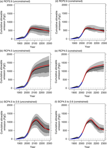
Figure 2 shows the time series of cumulative allowable carbon emissions. Except for the later times of RCP2.6 and SCP4.5 to 2.6, the ensemble mean of the calculated cumulative historical emissions (black curve) is slightly smaller than the harmonised emission scenarios (red curve) of RCP2.6 (van Vuuren et al., 2007), RCP4.5 (Smith and Wigley, 2006; Clarke et al., 2007; Wise et al., 2009) and SCP4.5 to 2.6. It is, however, consistent with our ensemble uncertainty range. Uncertainty is reduced by observational constraints for all scenarios.

Fig. 2 Time series of cumulative allowable emissions for period 1850–2300.

RCP2.6 (a), RCP4.5 (b) and SCP4.5 to 2.6 (c). The black curve is the ensemble mean, and the dark and light grey shades correspond to 68 (16–84 percentile) and 90 (5–95 percentile)% ranges respectively. The blue curve is the historical estimates of emissions (Carbon Dioxide Information Analysis Center: http://cdiac.ornl.gov/ftp/ndp030/global.1751_2009.ems). The red curves are harmonised RCP emissions (derived from MAGICC, documented in Meinshausen et al., 2011a). (d)–(f) are same as (a)–(c) but now for our constrained set of simulations using the eight observed datasets in Table 2.

Table 3 shows a comparison of cumulative emissions for RCPs 2.6 and 4.5 with the harmonised emission scenario (IAM) and CMIP5 models (Jones et al., 2013). Our results are consistent with the past (and IAM) emission and slightly smaller than IAM in the future both for RCPs 2.6 and 4.5. Our study, having a large number of ensemble members, includes extreme members and hence has large min-max ranges. However, the standard deviation is comparable (unconstrained case) with or 40% smaller (constrained case) than CMIP5 models. The uncertainty ranges include the IAM value. Table 4 shows a comparison of the emission reduction required to follow RCP2.6 for CMIP5 (Jones et al., 2013) and our study. Unlike CMIP5 models, our ensemble mean allowable emission in 2050s is significantly smaller than that of IAM (although large uncertainty ranges similar to CMIP5 models include the IAM value). This has potentially major policy implications. In our experiment, a larger reduction is required in 2050s relative to in 1990s to follow RCP2.6 pathway in comparison to the mean of the CMIP5 models and IAM.

Table 3  Comparison of cumulative fossil fuel emission with CMIP5 models

		CMIP5 models*		Our result**
Unit: PgC	Obs/IAM*	mean±σ	min–max range	mean±σ	min to max range
Historical	313	303±61	194–394	314±75	−77 to 577
				320±39
RCP2.6	325	322±106	189–469	282±103	−348 to 522
2006–2100				291±63
RCP4.5	786	831±155	194–394	738±173	−2.2 to 1199
2006–2100				728±82

*Jones et al. (2013), *upper: unconstrained, lower: constrained.

Table 4  Allowable fossil-fuel emissions for 1990s and 2050s for RCP2.6

Model	1990s emissions (PgC/yr)	2050s emissions (PgC/yr)	% reduction
CMIP5*	5.76±0.8	2.92±1.8	50
Our study**	6.01±1.3	1.79±1.7	70
	6.58±0.6	1.57±1.4	76
IAM***	6.35	2.39	62
Historical****	6.4±0.4

*Jones et al. (2013), **upper: unconstrained, lower: constrained, ***van Vuuren et al. (2007), ****Le Quéré et al. (2009).

3.2. Probability of the requirement for prolonged use of negative emissions

Figure 1 suggests that in order to achieve the RCP4.5 profile, the lowest mitigation scenario we consider, emissions are still required to be very low from 2100 onwards, and there is a non-trivial probability that negative global CO₂ emissions will be required both in the unconstrained and the constrained ensembles. After the late 22nd century, even the ensemble mean indicates a very low emissions rate of just 1.3 or 1.2 PgC/yr (unconstrained and constrained simulations for RCP4.5 respectively). Eliminating all anthropogenic emissions might prove difficult if burning of fossil fuels is needed to maintain food and water security, and this minimum level of emissions is sometimes termed the ‘emissions floor’ (Bowerman et al., 2011; Huntingford et al., 2012).

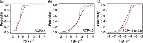
In Fig. 3, we present cumulative probabilities of average allowable emissions during the period 2151–2200 being less than different thresholds, and including negative global emissions. As can also be inferred from inspection of Fig. 1, for this period the cumulative probability curves are quite different between our unconstrained simulations (black curve) and constrained simulations (red curve). The red curves generally show larger probability changes for the same change in allowable emissions, consistent with uncertainty reduction. Almost all members require negative emission to follow the much higher mitigation scenario of RCP2.6 (Fig. 3a), and for SCP4.5 to 2.6 all members are required to have emissions of −2 PgC/yr or less to follow the pathway (Fig. 3c), indicating that, as expected, to follow them is far more difficult than to remain on RCP4.5. The median values are at −0.4, 1.5 and −4.7 PgC/yr for the unconstrained simulations, and for RCP2.6, RCP4.5 and SCP4.5 to 2.6, respectively. For the constrained simulations, these numbers become respectively −0.4, 1.6 and −4.4 PgC/yr. It should be noted that these are net emissions, and that with emission floors of 2 PgC/yr (for instance), −0.4 PgC/yr net will turn out to be −2.4 PgC/yr. To follow SCP4.5 to 2.6 net emissions of less than −4 PgC/yr are needed in many cases. This emphasises that the costs involved with later transition to a low concentration target are likely to be far higher during that transition period. Additionally, a period of carbon capture and storage that is of far higher magnitude than those involved in earlier transitions will be needed.

Fig. 3 The cumulative probability distribution for allowable emission thresholds when averaged over the period of years 2151–2200.

RCP2.6 (a), RCP4.5 (b) and SCP4.5 to 2.6 (c). The cumulative probability of these mean emissions being less than each threshold presented on the x-axis. Presented are the weighted probability for the unconstrained (black curve), and constrained ensembles using all variables in Table 2 (red curve).

3.3. Influence of the parameters on temperature trends and allowable emissions

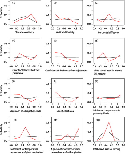
The relationship between the model parameters varied and the cumulative allowable emissions for 1850–2300 are presented in Fig. 4. The individual plots correspond to the 12 parameters presented in Table 1, which is the full set of parameters varied. For RCP4.5 and SCP4.5 to 2.6 the most influential parameter is climate sensitivity (black and blue in Fig. 4, Panel 1), while for RCP2.6 the aerosol (red, Panel 12) has slightly more correlation with cumulative emission. The correlation values are presented as colour-coded numbers in each panel. All parameters except the horizontal diffusivity of oceans and the coefficient of freshwater flux have effects, with 99% level significance (three ‘stars’), for cumulative allowable emissions for RCP4.5. From these, the soil respiration parameter has weaker influence in RCP2.6 and SCP4.5 to 2.6, the scenarios with less global warming.

Fig. 4 Relationship between the cumulative allowable emission (1850–2300) and variation in different parameter values.

RCP2.6 (red), RCP4.5 (black) and SCP4.5 to 2.6 (blue). Panels (1)–(12) are in the same order as Table 1. Numbers in plot areas are coefficients of correlation to parameter values (*/**/*** mean statistically significant at 90/95/99% levels). Plotted are the 512 members.

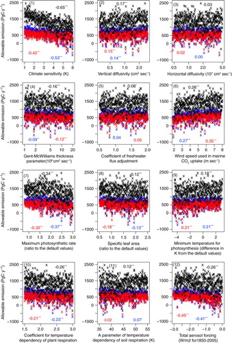
It is noticeable that besides the physical parameters, variation in the carbon-cycle-related parameters also make substantial contributions to altered estimates of allowable emissions. In some instances, the biogeochemical parameters have what appears initially to be a counter-intuitive influence. For example, higher maximum photosynthetic rate might suggest larger CO₂-draw-down and therefore higher allowable emissions, whereas Fig. 4 (Panel 7) suggests the opposite. This is likely because higher photosynthesis rates implies more terrestrial carbon stored on the ground for pre-industrial times, and so more terrestrial carbon becomes available for release to the atmosphere at higher temperatures. Also, as indicated in Tachiiri et al. (2012), once atmospheric concentrations of around 550 ppm are reached, then the high maximum photosynthetic rate constrains the photosynthesis through the effect of stomatal conductance, whereas at lower CO₂ concentrations that effect is less significant.

4. Other related outputs and discussion

4.1. Future temperature rise and related issues

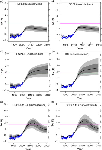
In Fig. 5, we present the spread of temperatures calculated in our ensemble for the different RCPs, and in the unconstrained and constrained cases. At year 2100, for RCPs, the average warming (black curves) is close to (unconstrained case) or slightly higher than (constrained case) that obtained from MAGICC harmonised calculations (Meinshausen et al., 2011c). For RCP2.6, we find the headline result that 89% of the ensemble members remain below the often-discussed 2K increase threshold. Unlike for allowable emissions, for all scenarios temperature uncertainty is not reduced by the observational constraint.

Fig. 5 Time series of global mean surface air temperature for period 1850–2300.

RCP2.6 (a), RCP4.5 (b) and SCP4.5 to 2.6 (c). The black curve is the ensemble mean, and the dark and light grey shades correspond to 68 (16–84 percentile) and 90 (5–95 percentile)% ranges respectively. The blue curve is the HadCRUT3 data (Brohan et al., 2006). Anomalies are from average of 1980–1999, and the horizontal magenta line is 2 K increase from the preindustrial (here average of 1850–1869). (d)–(f) are same as (a)–(c) but now for our constrained set of simulations using the eight observed datasets in Table 2.

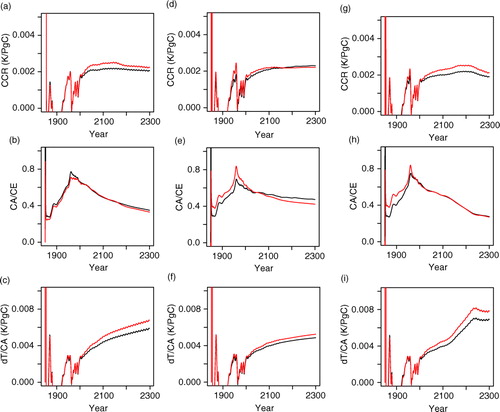
Allen et al. (2009), Matthews et al. (2009) and Meinshausen et al. (2009) suggested the ratio of temperature rise (dT) and cumulative carbon emission (C_E) keeps nearly constant due to the cancellation of two opposing nonlinear effects, airborne fraction and temperature rise for atmospheric CO₂ concentration (Raupach, 2013), and Matthews et al. (2009) call it Carbon Climate Response (CCR). Figure 6 presents the CCR, and also C_A/C_E (airborne fraction, C_A: airborne carbon) and dT/C_A (left-to-right) and for each scenario (top-to-bottom). In these simulations we also find that CCR keeps nearly constant by cancellation of the decreasing trend in C_A/C_E and the increasing trend in dT/C_A.

Fig. 6 Carbon Climate Response.

RCP2.6 (a–c), RCP4.5 (d–f) and SCP4.5 to 2.6 (g–i). The left (a, d, g), the central (b, e, h) and right (c, f, i) columns show Carbon Climate Response (ratio of temperature rise, dT, and cumulative emission (C_E), ratio of C_A (airborne carbon) and C_E (i.e. airborne fraction) and dT/C_A, respectively. Black and red lines are the unconstrained and the constrained ensemble average.

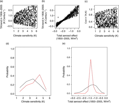
Figure 7a, b shows the influence of climate sensitivity and aerosol forcing on the trend in the global mean surface air temperature (TA trend). Figure 7a shows the interesting result that TA trend is not an effective constraint for climate sensitivity. However, in Fig. 7b, aerosol forcing has very strong effect on the TA trend. Figure 7c shows that all ensemble members of very low climate sensitivity (less than 1.5 K) have a large error in predicting historical temperature trend, implying that the real Earth system is less likely to have such a very low climate sensitivity. Figure 7d and e show how climate sensitivity and aerosol forcing are constrained by observation (transition from black curves to red curves). Figure 7d shows that for a distribution for climate sensitivity calculated based on weightings when using observational constraints (red curves), then this causes the peak of the distribution for climate sensitivity to be shifted to higher values between 4 and 5 K. This compares to the unconstrained-based distribution (black curve), that peaks at 3 K. We note that when we constrain our simulations with constraints from Table 2, but not using the historical fossil fuel record, then a much higher possibility remains of low climate sensitivity in tandem with small negative aerosol forcing. However inclusion of the fossil fuel emission record as a constraint, for our family of simulations, generally removes this possibility. It is still clearly not sufficient for very robust conclusions to be drawn about the tails of the distribution, even though the effective ensemble size of 10 (Table 2) is similar to ensemble sizes typical of the multi-model ensembles. Figure 7e, for aerosol forcing, shows in contrast how the comparison against observations, i.e. constrained ensemble, yields a significantly altered distribution shape. This focuses aerosol forcing almost exclusively to between −1.5 and −1.0 W/m² for 1850–2005. This is mainly the result of constraint by ocean heat content and by TA trends. We suggest that the main reason for our stronger constraint on aerosol radiative forcing, in comparison to that of for instance Harris et al. (2013), is through our use of multiple observation data. Our ability to tightly constrain the magnitude of the aerosol forcing with our model structure and comprehensive datasets is of very general interest to those analysing the climate system. To fully understand even contemporary warming implications of raised atmospheric greenhouse gas concentrations is difficult, in part due to uncertainty in the magnitude of offsetting cooling through raised aerosol concentrations. Our analysis has the potential to remove much of this difficulty. Effects of observational constraints on all parameters are presented in Appendix E.

Fig. 7 The dependence of temperature trend (warming between years 1906 to 2005), plotted against (a) climate sensitivity, (b) uncertainty in aerosol forcing. Also plotted, (c) is the cost (errors defined as absolute value of the difference) in TA trend vs climate sensitivity. Plotted are all of the 512 members. (d) and (e) are prior and posterior of climate sensitivity and aerosol forcing, in which black: unconstrained, red: constrained. Plotted are probabilities for bins of 0.1 K (d) and 0.5 W/m² (e) width.

4.2. Land and ocean carbon uptake and spatial distribution

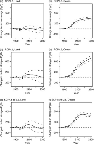
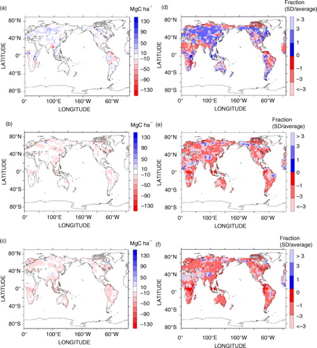
Figure 8 shows changes in global land and carbon storage (after constraint). The land becomes a carbon source in the near future for the major part of the ensemble [it should be noted, however, that the sensitivity of the land-borne carbon to the climate is around 20% higher in our model than the mean of the C4MIP models (γ_L in Appendix B)]. The ocean remains as a carbon sink for RCPs 2.6 and 4.5, but actually changes in to a carbon source in mid 22nd century for SCP4.5 to 2.6.

Fig. 8 Land and ocean carbon storage.

(a)–(c) are change in land carbon storage after constraint for RCP2.6, RCP4.5 and SCP4.5 to 2.6, respectively, and where a positive value implies a gain in carbon. The dark and light grey shades correspond to 68 (16–84 percentile) and 90 (5–95 percentile)% ranges respectively. (d)–(f) are change in ocean carbon storage for the scenarios.

The spatial resolving capability of our EMIC allows more elucidation of expected regional changes in carbon storage. Maps of land carbon uptake, for the constrained data for RCP4.5 and its associated uncertainty are presented in Fig. 9 (see Fig. F1 in Appendix for other two scenarios). For the change over period 2010–2100, on average, the Amazon is a major carbon source whilst most of other regions stay as net sinks (Fig. 9a). In the period 2100–2300, on average, the Amazon continues to be a source, whilst the northern high latitudes also become a large carbon source; only limited areas are net sink for the ensemble mean (Fig. 9b). This causes a net carbon loss by global land ecosystems, and hence explains the very small allowable emission in that period. However across our ensemble, most regions actually have greater uncertainty in terrestrial carbon store changes than the absolute values of the ensemble mean average. This is true both for 2010–2100 and 2100–2300 (Fig. 9c, d). Similar results are seen for the other scenarios too (Fig. F1 in Appendix).

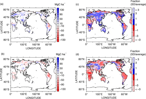
Fig. 9 Spatial distribution of the land carbon uptake.

Panel (a) is the weighted mean of land carbon uptake between 2010–2100 (i.e. year 2100 values minus year 2010 values), and (b) is land carbon uptake in 2100–2300. After constraint. Then panels (c) and (d) are relative uncertainty across the ensemble, calculated as SD/average in (a) and (b) respectively, presenting the extent of the consistency in the sign of change. When ∣SD/average∣ < 1, the sign of the change is considered be robust (note that the sign of ∣SD/average∣ simply presents that of average, as SD is always positive). Few grids are of robust signs for the change in 2010–2100, and even fewer grids are so in 2100–2300.

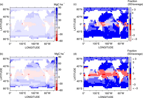
Figure 10 presents the same panels as Fig. 9, but for oceanic changes to carbon stocks (see Fig. F2 for RCP2.6 and RCP4.5 to 2.6). In 2010–2100 (Fig. 10a), carbon uptake by the ocean is positive with magnitude of 0–30 MgC/ha in most regions, and with larger magnitudes in the Southern Ocean and northern North Atlantic. Although there are some negative values in some equatorial regions, the positive uptake in most regions results in an overall global positive draw-down of atmospheric CO₂. In the period 2100–2300 (Fig. 10b), the regions with negative values expand, which is cancelled with high-latitudes having large positive values, and as such, globally the ocean remains a net sink of carbon, although reduced in magnitude compared to the earlier period. The relative uncertainty (SD/average) is larger in the equatorial regions in 2010–2100 (Fig. 10c) and such regions are expanded in the stabilised 2100–2300 period (Fig. 10d).

Fig. 10 Spatial distribution of the ocean carbon uptake (a): For 2010–2100, (b): 2100–2300, (c)(d): relative uncertainty (standard deviation/average). After constraint.

4.3. Notes on ensemble weights

The constraints to get the posterior (i.e. constrained) probability distributions are made by comparing different global sets of observations against outputs from our simulation ensemble. However, we do recognise that the parameter bounds and the global observations might not be completely independent, as expert judgment of model parameters may have been tuned implicitly considering some of the observations that we also use to weight our model simulations. That is, earlier understanding of the climate system implicit in the expert judgment of parameter ranges adopted in our Table 1 may have been informed to some extent by the observed values in our Table 2. We suggest that this might be in part why the use of constraints via the data of Table 2 did not reduce uncertainty in our predictions for global temperature change for each pathway as might have been expected.

The choice of weighting function (see Table 2 and Appendix D for the functions used in this study) also influences the result, but the main conclusion that the uncertainty in allowable emission, in particular before stabilisation, is decreased by the application of observational constraints will be robust for wide range of possible weighting functions. More discussion on ensemble weights is in Appendix G.

5. Conclusion

We have presented, possibly as a first of its kind, a large ensemble (order hundreds) of targeted perturbed-physics and perturbed-biogeochemical simulations, all with a climate model of significantly more complexity than a single point ‘box’ description. Parameter values defining key quantities known to affect both the climate system and the global carbon cycle have been selected to cover ranges based on present expert opinion. The parameter value ranges are also tested to ensure that we cover ranges implied by multiple climate modelling centres, which may also be regarded as a form of inclusion of existing opinion. Our EMIC ensemble, operating with such parameter perturbation, has then been used to estimate, with uncertainty bounds, allowable emissions associated with the low to medium-low atmospheric concentration (medium-high mitigation) pathways: RCP2.6, RCP4.5 and SCP4.5 to 2.6. We then take these simulations, and use a comprehensive set of contemporary measurements to assess the influence that additional data may exert on the ensemble, entrained in a way only possible with a geographically-resolving model system. This allows refined probabilities to be associated with each ensemble member, referred to as the ‘constrained’ ensemble.

Our findings are as follows. For both constrained and unconstrained projections, the mean of our spread of allowable CO₂ emissions is close to the standard ‘harmonised’ emission scenarios associated with each RCP. Further, our spread of allowable cumulative emissions is consistent with CMIP5 models (Jones et al., 2013). By applying the constraints of Table 2, we find that the uncertainty in allowable emissions reduces from being of similar magnitude to CMIP5, down to time-evolving ranges approximately 40% smaller over the period years 2006 to 2100. However, the influence of the observational comparison places less constraint on the range of allowable emissions for the period after climate stabilisation. Additionally there is a possibility that negative net emissions are eventually required and even to follow the RCP4.5 scenario. This is despite RCP4.5 being the most moderate scenario in terms of mitigation that we consider here. Negative emissions would imply a global requirement for large-scale carbon capture and storage, most likely in addition to deep cuts in emissions. As expected, heavier mitigation scenarios of RCP2.6 and SCP4.5 to 2.6 require harsher emission reductions. In particular, to follow a later transition to RCP2.6 concentrations (SCP4.5 to 2.6), a low (negative) emissions reaching approximately −5 PgC/yr will be required. Possible negative emissions are predicted in part because, for many parameter sets, the land will turn into a carbon source within the 21st century. In most instances the ocean, however and when considered globally, is predicted to remain as a sink of atmospheric carbon dioxide in all simulations except for the period with a strong overshoot in CO₂ concentration in SCP4.5 to 2.6. Whilst the detail of the distribution, such as tail, can be influenced by sampling and weighting methods, these general results are expected to be robust.

Of the parameters varied, climate sensitivity has the most significant impact on allowable emissions for RCP4.5 and SCP4.5 to 2.6, while for RCP2.6 aerosol forcing is most effective. This demonstrates the importance of thermal climate-change feedbacks on the land and ocean stores of carbon, altering their ability to ‘draw-down’ (or otherwise) atmospheric CO₂. As might be expected, some more direct carbon-cycle related parameters also have a significant effect on allowable emissions. We have been able to investigate this further, as our EMIC allows for the provision of geographical information. We find that eventually both the Amazon and northern high latitude (of land) show significant carbon release back in to the atmosphere, while the Southern Ocean and northern North Atlantic generally have very strong levels of carbon uptake.

In our study, distributions of global mean temperature rise are also calculated across the unconstrained and constrained ensembles, and again corresponding to the three RCP pathways we have analysed. However, unlike where we could use the emission observation to refine allowable emissions, the trade-off between climate sensitivity and aerosol forcing in our study period still prevented us from achieving a reduced spread in predicted levels of future global warming – aerosol radiative forcing is effectively constrained, but not enough to narrow the distribution of climate sensitivity. It is also possible that more detailed constraints on carbon cycle can significantly change the distribution of the constrained climate sensitivity.

The careful fusion of models with data is critical to enhancing understanding of the climate system, and including explanation of contemporary and past observations. However for planning purposes, of more importance is that such activity aids in making future predictions more robust. When performed in tandem with ensembles of simulations, it can at the minimum provide probabilistic estimates of future change as demanded by policymakers. However until now, computational requirement has made it extremely difficult to make ensembles of more complex climate models, preventing the entrainment of emerging datasets that might have strong regional differences. The techniques reported here are a significant step towards eventual ensemble operation of full complexity climate models (i.e. even higher complexity and resolution than our EMIC), especially as even more computational resource becomes available and including the potential use of cloud computing services (Huntingford, 2013). This will then allow, for instance, a rigorous depiction of the spatially very heterogeneous sulphate forcing, and its uncertainties which are known to be large (Forster et al., 2007).

We have presented allowable emissions implications for three key medium-to-high mitigation RCP trajectories of future altered atmospheric gas concentrations. To achieve the atmospheric concentrations of these scenarios, CO₂ emissions must peak soon before major on-going reductions. This is as expected, but here presented with a full representation of uncertainty. However, despite the use of contemporary measurements to constrain simulations further and thus beyond the expert-opinion bounds on key parameters, our uncertainty bounds on levels of warming for all scenarios considered do remain larger than is ideal for policy planning purposes. Hence we look forward to repeating these analyses at a future date with a higher-resolution model and slightly longer datasets, and to see the influence this might have on ensemble temperature spread. Our results have been possible using an ensemble modelling structure with a systematic mechanism to routinely entrain emerging datasets. Some of these datasets are of complexity levels that cannot be entrained in to global ‘box’ formulations. We hope this analysis is a first step towards providing routine and significantly more refined uncertainty bounds around policy-specific climate change questions with the benefits that more complex climate models provide.

6. Acknowledgements

The authors wish to thank the developers of MIROC and MIROC-lite. This work is supported by Innovative Program of Climate Change Projection for the 21st Century and Program for Risk Information on Climate Change (of the Ministry of Education, Culture, Sports, Science and Technology, MEXT, Japan). The super-computing resource was provided by Japan Agency for Marine-Earth Science and Technology. CH is grateful for support from the CEH science budget fund.

Appendix

A: Parameters with non-flat priors

A1 Climate sensitivity

Multiple studies have categorised the available estimates of climate sensitivity, as this is a fundamental parameter to characterise global warming. In most instances, any distribution from across-model ensembles has been found to be asymmetric. Hence it is not possible to rule out quite high values (sometimes called the “fat upper tail”). In order to consider a more realistic probability density function (PDF) for climate sensitivity than a uniform one, we adopt a beta function. This has an asymmetric shape and is easy to define, with only two parameters. This is used to represent the prior. The definition of a beta function is:

and when it is used as a PDF in variable x (here climate sensitivity), it is given as:

We fitted this to the IPCC AR4's “likely” (i.e. of 66% confidence) range of 2–4.5°C, thus we use the parameters B(1.8,2.2) which actually gives positive numbers over range 1–6°C (Fig. A1 and Fig. A2). This results in a distribution which is maximised at around 3°C and which assigns roughly 15% probability to the sensitivity lying outside either end of the IPCC likely range, resulting that 69% is between 2 and 4.5 K.

Fig. E1 Prior and posterior probability distribution of 12 parameters. Black: prior (unconstrained), red: posterior (after constrained by observation data). X-axis is normalised to the perturbation range (logarithmic scales for 2–4). Priors are flat for all parameters but climate sensitivity and aerosol for which non-flat distributions presented in Appendix A are used. Plotted are probabilities for bins of 0.2 (i.e. one fifth of the pertubed range) width.

A2 Aerosol

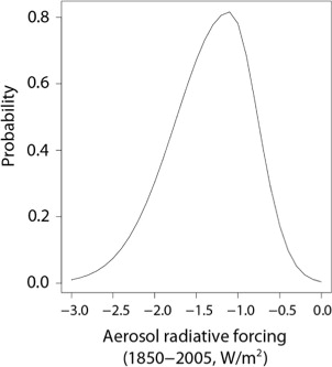
In Hegerl et al. (2007), the total (direct and indirect) aerosol effect is −3.00 to 0.00 W/m² for 1750–2005. In the forcing for the past associated with RCP scenarios, aerosol forcing for 1765–2005 and for 1850–2005 is about −1.1 W/m² and −1.0 W/m². In this study, by multiplying with 0–3, the aerosol forcing for 1850–2005 is perturbed as −3.0–0.0 W/m².

To mimic the PDF of Hegerl et al. (2007), we use a combination of two Gaussian functions: N(−1.1,0.64²)×1.29 for −3≤RF≤−1.1 (W/m²) and N(−1.1, 0.34²)×0.69 for −1.1 < RF≤0 (W/m²) (where RF is radiative forcing, and the coefficients are determined to have the two functions connected at −1.1, and to make the integral to be 1).

Fig. F1 Spatial distribution of the change in land carbon storage for RCP2.6 and SCP4.5 to 2.6. Panel (a) is the weighted mean of land carbon uptake between 2010 and 2100 (i.e. year 2100 values minus year 2010 values), and (b) is land carbon uptake in 2100–2300 for RCP2.6. (c) is land carbon uptake in 2100–2300 for SCP4.5 to 2.6. Then panels (d)–(f) are relative uncertainty across the ensemble, calculated as SD/average in (a)–(c) respectively. After constraint.

Although Hegerl et al. (2007) provide quantitative information only for the sum of the aerosol's direct and the first kind indirect (i.e. cloud albedo) effects, there are many other kinds of indirect effects (Lohmann and Feichter, 2005), such as cloud lifetime effect which is often called the second kind of indirect effect. The total shortwave aerosol forcing is estimated to be −1.5±0.5 Wm² or −1.2±0.4 Wm² by two different methods (Quaas et al., 2009) and the latter is close to a recent estimate (−1.17 Wm²; −0.74 to −1.44 Wm²) by Shindell et al. (2013). Although we use the prior distribution based on the direct and the first indirect aerosol effects, it should be interpreted that the posterior distribution after observational constraint gives that of the total (i.e. including direct and all kinds of indirect) aerosol forcing.

B: The basis of the parametric uncertainty explored using JUMP-LCM

Fig. F2 Ocean carbon uptake (a) for 2010–2100, (b) 2100–2300 for RCP2.6, (c) 2100–2300 for SCP4.5 to 2.6, (d)–(f) relative uncertainty (standard deviation/average) for (a)–(c). After constraint.

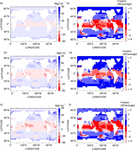
Fig. A1 The beta distribution with values B(1.8, 2.2), used to represent the asymmetric climate sensitivity's probability distribution.

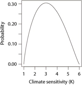
Fig. A2 The distribution of aerosol represented using a combination of two normal functions.

Recent work by Yokohata et al. (2011) analysed the CMIP3 multi-model ensemble and found the ensemble has plausible range, which gives us reason to hope that existing ESMs, developed by similar model centres and having common or similar physics with CMIP3 models, also give plausible ranges in their future dispersion. We use such a multi-model ensemble (the Coupled Carbon Cycle Climate Model Intercomparison Project; C4MIP, Friedlingstein et al., 2006), combined with expert opinion of the JUMP-LCM model developers, as a guide to key parameter ranges. The ranges are originally based on those reported in previous studies (Tachiiri et al., 2010, 2012) but subsequently shifted to cover bounds more similar to those implicit in the C4MIP (Friedlingstein et al., 2006) set of full-complexity climate-carbon cycle simulations. The C4MIP simulations capture model behaviour in terms of five key effective parameters: linear transient climate sensitivity (α), sensitivity of land and ocean carbon storage to the change in carbon content in atmosphere (β_L and β_O) and sensitivity of land and ocean carbon storage to the change in global mean surface air temperature (γ_L and γ_O). The ranges for our equivalent effective parameters are given in Table B1 (based on parameter variations in JUMP-LCM; see Table 1). The results broadly span the range of C4MIP's results (Table B1). This is an encouraging outcome as we cannot expect to fully encapsulate all model behaviours found in a structurally diverse multi-model ensemble.

The difference between the ranges of the five effective parameters from the C4MIP simulations and from our modelling system is small, but there still remain non-negligible differences. Particularly, the smaller average and standard deviation in β_L result that our model explores the lower β_L (leading to less future carbon uptake) portion of the C4MIP range. The original parameter perturbation range before tuning for C4MIP models is presented in Table B2. To achieve this comparability, except for equilibrium climate sensitivity (which are fixed, as presented in Table 1) and aerosol forcing (not used, following the C4MIP protocol), the tuning is carried out heuristically using a small ensemble with 20 members. We compared these ranges of α, β and γ against their equivalent numbers across the C4MIP range of climate-carbon cycle simulations. An iterative process is then made across our parameter ranges in Table B2 until our α, β and γ values coincided more closely with the C4MIP ranges, and this modification is the difference between our Table B2 and Table 1. These parameter ranges and probabilities define our “unconstrained” experiments. The parameters varied, and their ranges, are presented in Table 1. More details regarding the parameters are given in Appendix C.

Table B1 . Feedback parameters compared to the C4MIP models

	Unit	This study	C4MIP
α	K/ppm	0.0054±0.0013	0.0061±0.0012
βL	PgC/ppm	1.1±0.3	1.3±0.6
βO	PgC/ppm	1.2±0.3	1.1±0.2
γL	PgC/K	−97±75	−79±44
γO	PgC/K	−33±11	−31±16

Parameters presented (Friedlingstein et al., 2006), are linear transient climate sensitivity (α), sensitivity of land and ocean carbon storage to atmospheric CO₂ concentration change (β) and to temperature change (γ). “l” and “o” are land and ocean. The ± one SD of 20 members (in a small ensemble) and also for C4MIP models are presented.

Table B2 . Original parameter perturbation ranges before the tuning for the C4MIP models

Parameters	Original perturbation range
Climate sensitivity	(1–6 K)
Vertical diffusivity	0.5–2.0×default
Horizontal diffusivity	0.5–5.0×default
Gent-McWilliams thickness parameter (a)	1–10×10^6 cm^2/s
Magnitude of freshwater flux adjustment	0.5–2.0×Oort's values (b)
Wind speed used in marine CO2 uptake	1–6 m/s
Maximum photosynthetic rate	0.8–2.0×default
Specific leaf area	0.5–1.5×default
Minimum temperature for photosynthesis	−3.0~ + 3.0°C of default
Coefficient for temperature dependency of plant's respiration	1.5–3.0
A parameter of temperature dependency of soil respiration	40–60 K
Total aerosol forcing	–

Ranges are based on Tachiiri et al. (2010) Tachiiri et al. (2012). (a) Gent and McWilliams (1990). (b) Oort (1983).

C: Parameters varied

A detailed description of the 12 varied parameters are as follows.

The first parameter is climate sensitivity. Although in a full-complexity GCM this is not an (effective) parameter which can be easily controlled, in an EMIC this can be controlled relatively easily. For the detail of how climate sensitivity is controlled in our model, please see Tachiiri et al. (2010).

The next four parameters varied are related to ocean physics. The (initial) vertical and horizontal diffusivities are depth dependent. The Gent-McWilliams parameter (Gent and McWilliams, 1990) parameterises the sub-grid scale eddy effect. The magnitude of the freshwater flux adjustment is an EMIC specific parameter. As many EMICs cannot represent well the freshwater transportation between Pacific and Atlantic oceans, it is necessary to add artificial movement between them. The parameter is considered as a ratio of modelled values to the estimates by Oort (1983) providing values for some latitudinal bands.

The sixth parameter, wind speed used in marine CO₂ uptake, is also EMIC specific. As described in Orr (2000), air-sea CO₂ flux is calculated as a function of the wind speed. In GCMs simulated wind speed is used, but in many EMICs including MIROC-lite, simulated wind speed in each grid cell can contain large biases compared to actual values, and often a fixed value is used. Given that changing wind speed is only way to obtain plausible ranges in marine carbon response to concentration and to temperature change similar to those of C4MIP models, then we perturbed the wind speed used in air-sea CO₂ flux calculation. These six parameters so far are selected considering Tachiiri et al. (2010) and their assessment of key parameters of importance.

The 7–11th parameters are related to terrestrial carbon cycle, and this time selected based on another study (Tachiiri et al., 2012) which in turn made an assessment of the twelve most important parameters for the carbon cycle. In Tachiiri et al. (2012), the four parameters of maximum photosynthetic rate, specific leaf area, minimum temperature for photosynthesis and a soil respiration parameter had correlation of 99% level significance with both CO₂ and temperature response of the land surface, characterised by effective parameters β_L and γ_L. When their effects are combined, the temperature dependency of plant respiration has largest correlation to change in terrestrial carbon storage in RCP4.5 scenario (Tachiiri et al., 2012).

The 12th and last parameter varied is aerosol forcing. Information on parameter ranges taken from the two key references (Tachiiri et al. 2010, 2012) are presented be in Table B2.

D: Data for constraint

For the physical climate system, we use the trend in surface air temperature in 1906–2005 (Trenberth et al., 2007), the trend in ocean heat content (OHC) of 0–700 m depth during 1969–2003 (Domingues et al., 2008; Ishii and Kimoto, 2009; Levitus et al., 2009), Atlantic meridional overturning circulation (derived from Lumpkin and Speer, 2010; Smethie Jr. and Fine, 2001; Ganachaud, 2003; Talley et al., 2003), present day air temperature (2 dimensional, NCEP/NCAR reanalysis; Kistler et al., 2001), and present sea temperature/salinity (3 dimensional, World Ocean Atlas, http://www.esrl.noaa.gov/psd/data/gridded/data.nodc.woa98.html). We also use observations relating to carbon cycle component of the model: implied fossil fuel CO₂ emissions in 1980s, 1990s and 2000–2008 (Le Quéré et al., 2009) and present day net primary production (Zheng et al., 2003).

The assumed probabilistic function is a t-distribution for trends in both global mean surface air temperature and OHC, and Gaussian for other data. For the two dimensional (i.e. spatial) data, we used weights designed along similar principles to those used by Murphy et al. (2004). That is, we first calculated the ratio of the mean square error of each ensemble member to the spatial variance of the observed data (for all the globe), and using this ratio (called CPI’ here, due to the similarity to Climate Prediction Index, or CPI; Murphy et al., 2004), the weight (W) is calculated as W=exp[–CPI’/2]. We normalised all weights across the ensemble, so that they add up to unity, with each observed variable having equal weight. For the emissions data, we calculated the weight as the geometric mean of the values for the three decades, and for the sea temperature and salinity, we calculated the geometric means of the four ocean layers.

E: Constraint on parameters

The distributions of the varied parameters are also influenced by the observational constraints. Figure E1 presents the posterior distribution of each parameter. The weighted distribution is concentrated on either side of the parameter perturbation range for some parameters. For example, a temperature dependency parameter of soil respiration (panel 11) has high probability of high parameter values, while oceanic vertical diffusivity (panel 2) and parameter of freshwater flux adjustment (panel 5) are more likely to have low parameter values.

F: Spatial distribution of carbon uptake for RCP2.6 and SCP4.5 to 2.6 ( Figs. F1 and Fig. F2 )

G: More discussion on the ensemble weights

The use of constraints should be made with some caution for a couple of additional reasons. Some combinations of model parameters may correspond to good predictive capability for present-day, but will subsequently be found to perform poorly for prediction at significantly altered atmospheric gas concentrations. This is because some features or parameterisation of a climate model might not matter for current levels of atmospheric CO₂ concentrations, but do become much more important (and thus need correct parameterisation) for significantly higher CO₂ concentrations. Conversely, it is possible to weight down a particular simulation based on contemporary measurements, but which actually has good predictive capability for the future. For those issues, Knutti et al. (2010) pointed out a weighting metric is most powerful if it is relatively simple but statistically robust, if the results are not strongly dependent on the detailed specifications of the metric and other choices external to the model (e.g. the forcing) and if the results can be understood in terms of known processes. We hope our methodology at least partially fulfils these objectives.

There remains significant interest in the upper tail of PDF of climate sensitivity, corresponding to what might be low probability events, but potentially very difficult for society to adapt to. In order to assess the effect of changing the upper bound for the climate sensitivity (CS) range, we investigated the sensitivity of the results with RCP4.5 to the cut off of the upper tail of the beta distribution (B (1.8,2.2)) at 5.0 and 5.5 K (i.e. zero probability of CS > 5.0 and >5.5 K, respectively). For the unconstrained case the influence is very small; this is not surprising as the weights given to high CS members are small. For the constrained case, we have a rather small effective ensemble size which introduces significant sampling noise. That effect was not observed for temperature, but had some influence on allowable emission. After multiplying 8 weights, the biggest weight for one ensemble member in our experiment was 0.22 (RCP2.6) or 0.24 (RCP4.5 and SCP4.5 to 2.6), depending on the emission in 2006–2008, and thus while the main results of the unconstrained case are robust to maximum cut-off of climate sensitivity, the constrained case is less robust. These results are summarised in Table G1.

Table G1 . Result of the sensitivity tests for climate sensitivity with RCP4.5

	Atmospheric temperature (K)		Allowable emission (PgC/yr)
Cut-off point	Unconstrained	Constrained	Unconstrained	Constrained
6.0 K (original)	1.2–3.4	1.3–3.3	7.4–13.7	9.9–13.0
5.5 K	1.2–3.4	1.5–3.3	7.4–13.7	9.5–12.5
5.0 K	1.2–3.3	1.5–3.3	7.7–13.9	9.8–12.5

The 5–95th percentiles for the peak periods are presented. Temperatures are anomaly from 1980 to 99.

References

- Allen M. R , Frame D. J , Huntingford C , Jones C. D , Lowe J. A , co-authors . Warming caused by cumulative carbon emissions towards the trillionth tonne. Nature. 2009; 458: 1163–1166.
- Annan J. D , Hargreaves J. C . On the generation and interpretation of probabilistic estimates of climate sensitivity. Clim. Change. 2009; 104: 423–436.
- Arora V. K , Boer G. J , Friedlingstein P , Eby M , Jones C. D , co-authors . Carbon-concentration and carbon-climate feedbacks in CMIP5 Earth system models. J. Clim. 2013. 26, 5289–5314. DOI: 10.1175/JCLI-D-12-00494.1.
- Arora V. K , Scinocca J. F , Boer G. J , Christian J. R , Denman K. L , co-authors . Carbon emission limits required to satisfy future representative concentration pathways of greenhouse gases. Geophys. Res. Lett. 2011; 38: 05805.
- Bodman R. W , Rayner P. J , Karoly D. J . Uncertainty in temperature projections reduced using carbon cycle and climate observations. Nat. Clim. Change. 2013. 3, 725–729. DOI: 10.1038/nclimate1903.
- Bowerman N. H. A , Frame D. J , Huntingford C , Lowe J. A , Allen M. R . Cumulative carbon emissions, emissions floors and short-term rates of warming: implications for policy. Philos. Trans. R. Soc. A. 2011; 369: 45–66.
- Brohan P , Kennedy J. J , Harris I , Tett S. F. B , Jones P. D . Uncertainty estimates in regional and global observed temperature changes: a new dataset from 1850. J. Geophys. Res. 2006; 111: 12106.
- Clarke L , Edmonds J , Jacoby H , Pitcher H , Reilly J , co-authors . Scenarios of Greenhouse Gas Emissions and Atmospheric Concentrations. Sub-report 2.1A of Synthesis and Assessment Product 2.1 by the U.S. Climate Change Science Program and the Subcommittee on Global Change Research.
- Forster P , Ramaswamy V , Artaxo P , Berntsen T , Betts R , co-authors . Solomon S , Qin D , Manning M , Chen Z , Marquis M , co-authors . Changes in atmospheric constituents and in radiative forcing. Climate Change 2007: The Physical Science Basis. Contribution of Working Group I to the Fourth Assessment Report of the Intergovernmental Panel on Climate Change. 2007; Cambridge, UK and New York, NY, USA: Cambridge University Press. 129–234.
- Friedlingstein P , Cox P , Betts R , Bopp L , von Bloh W , co-authors . Climate-carbon cycle feedback analysis, results from the C4MIP model intercomparison. J. Clim. 2006; 19: 3337–3353.
- Ganachaud A . Large-scale mass transports, water mass formation, and diffusivities estimated from World Ocean Circulation Experiment (WOCE) hydrographic data. J. Geophys. Res. 2003; 108(C7): 3213.
- Gent P. R , McWilliams J. C . Isopycnal mixing in ocean circulation models. J. Phys. Oceanogr. 1990; 20: 150–155.
- Gregory J. M , Jones C. D , Cadule P , Friedlingstein P . Quantifying carbon cycle feedbacks. J. Clim. 2009; 22: 5232–5250.
- Hajima T , Ise T , Tachiiri K , Kato E , Watabnabe S , Kawamiya M . Climate change, allowable emission, and earth system response to representative concentration pathway scenarios. J. Meteorol. Soc. Jpn. 2012; 90(3): 417–434.
- Harris G. R , Sexton D. M. H , Booth B. B. B , Collins M , Murphy J. M . Probabilistic projections of transient climate change. Clim. Dynam. 2013. 40, 2937–2972. DOI: 10.1007/s00382-012-1647-y.
- Hegerl G. C , Zwiers F. W , Braconnot P , Gillett N. P , Luo Y , co-authors . Solomon S . Understanding and attributing climate change. Climate Change 2007: The Physical Science Basis. Contribution of Working Group I to the Fourth Assessment Report of the Inter-governmental Panel on Climate Change. 2007; Cambridge, UK and New York, NY, USA: Cambridge University Press. 663–745.
- Houghton R. A , van der Werf G. R , DeFries R. S , Hansen M. C , House J. I , co-authors . Chapter G2 Carbon emissions from land use and land-cover change. Biogeosci. Discuss. 2012; 9: 835–878.
- Huntingford C . Climate projection: refining global warming projections. Nat. Clim. Change. 2013; 3: 704–705.
- Huntingford C , Lowe J. A , Gohar L. K , Bowerman N. H. A , Allen M. R , co-authors . The link between a global 2°C warming threshold and emissions in years 2020, 2050 and beyond, Environ. Res. Lett. 2012; 7(1): 014039.
- Ishii M , Kimoto M . Reevaluation of historical ocean heat content variations with time-varying XBT and MBT depth bias corrections. J. Oceanogr. 2009; 65: 287–299.
- Ito A , Oikawa T . A simulation model of the carbon cycle in land ecosystems (Sim-CYCLE): a description based on drymatter production theory and plot-scale validation. Ecol. Model. 2002; 151: 143–176.
- Jones C. D , Robertson E , Arora V , Friedlingstein P , Shevliakova E , co-authors . 21st Century compatible CO2 emissions and airborne fraction simulated by CMIP5 earth system models under 4 representative concentration pathways. J. Clim. 2013. 26, 4398–4413. DOI: 10.1175/JCLI-D-12-00554.1.
- K-1 model developers. K-1 Coupled GCM (MIROC) Description, K-1 Technical Report No. 1. 2004. Online at: http://www.ccsr.u-tokyo.ac.jp/kyosei/hasumi/MIROC/tech-repo.pdf .
- Kistler R , Kalnay E , Collins W , Saha S , White G , co-authors . The NCEP-NCAR 50-year reanalysis: monthly means CD-ROM and documentation. Bull. Am. Meteorol. Soc. 2001; 82: 247–268.
- Knutti R , Abramowitz G , Collins M , Eyring V , Gleckler P. J , co-authors . Stocker T. F , Qin D , Plattner G.-K , Tignor M , Midgley P. M . In: Meeting Report of the Intergovernmental Panel on Climate Change Expert Meeting on Assessing and Combining Multi Model Climate Projections. 2010; University of Bern, Bern, Switzerland: IPCC Working Group I Technical Support Unit. Online at: http://www.ipcc-wg2.gov/meetings/EMs/IPCC_EM_MultiModelEvaluation_MeetingReport.pdf .
- Lenton T. M . Land and ocean carbon cycle feedback effects on global warming in a simple earth system model. Tellus. 2000; 52B: 1159–1188.
- Le Quéré C , Raupach M. R , Canadell J. G , Marland G , Bopp L , co-authors . Trends in the sources and sinks of carbon dioxide. Nat. Geosci. 2009; 2: 831–836.
- Levitus S , Antonov J. I , Boyer T. P , Locarnini R. A , Garcia H. E , co-authors . Global ocean heat content 1955–2008 in light of recently revealed instrumentation problems. Geophys. Res. Lett. 2009; 36: 07608.
- Lohmann U , Feichter J . Global indirect aerosol effects: a review. Atmos. Chem. Phys. 2005; 5: 715–737.
- Lumpkin R , Speer K . Global ocean meridional overturning. J. Phys. Oceanogr. 2010; 37: 2550–2562.
- Matthews H. D , Gillett N. P , Stott P. A , Zickfeld K . The proportionality of global warming to cumulative carbon emissions. Nature. 2009; 459: 829–832.
- Meinshausen M , Meinshausen N , Hare W , Raper S. C. B , Frieler K , co-authors . Greenhouse-gas emission targets for limiting global warming to 2°C. Nature. 2009; 458: 1158–1162.
- Meinshausen M , Raper S. C. B , Wigley T. M. L . Emulating coupled atmosphere-ocean and carbon cycle models with a simpler model, MAGICC6 – Part 1: model description and calibration. Atmos. Chem. Phys. 2011a; 11: 1417–1456.
- Meinshausen M , Smith S. J , Calvin K. V , Daniel J. S , Kainuma M , co-authors . The RCP greenhouse gas concentrations and their extension from 1765 to 2300. Clim. Change. 2011b; 109: 213–241.
- Meinshausen M , Wigley T. M. L , Raper S. C. B . Emulating atmosphere-ocean and carbon cycle models with a simpler model, MAGICC6 – Part 2: applications. Atmos. Chem. Phys. 2011c; 11: 1457–1471.
- Moss R , Edmonds J , Hibbard K , Manning M , Rose S , co-authors . The next generation of scenarios for climate change research and assessment. Nature. 2010; 463: 747–756.
- Murphy J. M , Sexton D. M. H , Barnett D. N , Jones G. S , Webb M. J , co-authors . Quantifying uncertainties in climate change from a large ensemble of general circulation model predictions. Nature. 2004; 430: 768–772.
- Oka A , Tajika E , Abe-Ouchi A , Kubota K . Role of the ocean in controlling atmospheric CO2 concentration in the course of global glaciations. Clim. Dyn. 2011; 37: 1755–1770.
- Oort A. H . Global atmospheric circulation statistics, 1958–1973. NOAA Prof Pap. 1983; 14: 180.
- Orr J , Najjar R , Sabine C , Joos F . Abiotic-HOWTO Revision: 1.16. 2000. Online at: http://www.cgd.ucar.edu/oce/klindsay/ocmip/HOWTO-Abiotic.pdf .
- Quaas J , Ming Y , Menon S , Takemura T , Wang M , co-authors . Aerosol indirect effects—general circulation model intercomparison and evaluation with satellite data. Atmos. Chem. Phys. 2009; 9: 8697–8717.
- Raupach M. R . The exponential eigenmodes of the carbon-climate system, and their implications for ratios of responses to forcings. Earth Syst. Dynam. 2013; 4: 31–49.
- Shindell D. T , Lamarque J.-F , Schulz M , Flanner M , Jiao C , co-authors . Radiative forcing in the ACCMIP historical and future climate simulations. Atmos. Chem. Phys. 2013; 13: 2939–2974.
- Smethie W. M Jr. , Fine R. A . Rates of North Atlantic Deep Water formation calculated from chlorofluorocarbon inventories. Deep-Sea Res. PT1. 2001; 48: 189–215.
- Smith S. J , Wigley T. M. L . Multi-gas forcing stabilization with the MiniCAM. Energ. J. 2006 Special Issue No. 3 373–391.
- Tachiiri K , Hargreaves J. C , Annan J. D , Oka A , Abe-Ouchi A , co-authors . Development of a system emulating the global carbon cycle in earth system models. Geosci. Model Dev. 2010; 3: 365–376.
- Tachiiri K , Ito A , Hajima T , Hargreaves J. C , Annan J. D , co-authors . Nonlinearity of land carbon sensitivities in climate change simulations. J. Meteorol. Soc. Jpn. 2012; 90A: 271–276.
- Talley L. D , Reid J. L , Robbins P. E . Data-based meridional overturning streamfunctions for the global ocean. J. Clim. 2003; 16: 3213–3226.
- Taylor K. E , Stouffer R. J , Meehl G. A . A summary of the CMIP5 experimental design. 2009. Online at: http://cmip-pcmdi.llnl.gov/cmip5/docs/Taylor_CMIP5_22Jan11_marked.pdf .
- Trenberth K. E , Jones P. D , Ambenje P , Bojariu R , Easterling D , co-authors . Solomon S . Observations: surface and atmospheric climate change. Climate Change 2007: In The Physical Science Basis. Contribution of Working Group I to the Fourth Assessment Report of the Intergovernmental Panel on Climate Change. 2007; Cambridge, UK and New York, NY, USA: Cambridge University Press. 235–336.
- van Vuuren D , den Elzen M , Lucas P , Eickhout B , Strengers B , co-authors . Stabilizing greenhouse gas concentrations at low levels: an assessment of reduction strategies and costs. Clim. Change. 2007; 81(2): 119–159.
- Wise M. A , Calvin K. V , Thomson A. M , Clarke L. E , Bond-Lamberty B , co-authors . Implications of limiting CO2 concentrations for land use and energy. Science. 2009; 324: 1183–1186.
- Yokohata T , Annan J. D , Hargreaves J. C , Jackson C. S , Tobis M , co-authors . Reliability of multi-model and structurally different single-model ensembles. Clim. Dyn. 2011; 39(3–4): 599–616.
- Yoshikawa C , Kawamiya M , Kato T , Yamanaka Y , Matsuno T . Geographical distribution of the feedback between future climate change and the carbon cycle. J. Geophys. Res. 2008; 113: 03002.
- Zheng D. L , Prince S. D , Wright R . NPP Multi-Biome: gridded estimates for selected regions worldwide, 1989–2001, R1. 2003. Online at: http://daac.ornl.gov/cgi-bin/dsviewer.pl?ds_id=614, the Oak Ridge National Laboratory Distributed Active Archive Center, Oak Ridge, Tennessee, U.S.A..