Mass transfer velocity across the breaking air–water interface at extremely high wind speeds

Abstract

Mass transfer velocity k _L across the wind-driven air–water interface was estimated at extremely high wind speeds (up to U ₁₀=70 m s⁻¹) in a high-speed wind-wave tank by measuring changes in CO₂ concentration in the water. In addition, the volume flux of dispersing droplets lost from the tank and the wave height were measured. k _L increases drastically with wind speed at extremely high wind speeds. The volume flux of dispersing droplets begins to increase drastically and the mean height of significant waves changes its rate of increase at almost the same wind speed as that at which the rate of increase of k _L changed. These results suggest that intense wave breaking occurs at extremely high wind speeds and it has significant effects on mass transfer. k _L is well correlated with the free-stream wind speed for both present laboratory and previous field measurements in the low and moderate wind speed regions. Present k _L agrees well with the conventional correlation curves proposed by Wanninkhof (1992), Wanninkhof and McGillis (1999) and Wanninkhof et al. (2009) for low and moderate free-stream wind speeds. However, for extremely high free-stream wind speeds, the present data deviate upward from the correlation curves of Wanninkhof (1992) and Wanninkhof and McGillis (1999) and approach to that of Wanninkhof et al. (2009) as the wind speed increases. This indicates that the correlation curve of Wanninkhof et al. (2009) is more appropriate for the correlation between k _L and free-stream wind speed than those of Wanninkhof (1992) and Wanninkhof and McGillis (1999) in extremely high wind speed region.

• air–sea gas exchange
• air–sea interaction
• tropical cyclone
• wind wave
• breaking wave

View correction statement:

ERRATUM

A Erratum has been published for this paper. Please see http://www.tellusb.net/index.php/tellusb/article/view/25233

1. Introduction

To predict future atmospheric temperatures, it is of great importance to precisely estimate the global carbon cycle. One of the important issues is to accurately predict mass transfer rate of greenhouse gases across the air–sea interface between atmosphere and oceans which cover about 70% of the surface of the earth. These days, some researchers have suggested that tropical cyclones may significantly affect spatial and temporal variations in CO₂ flux between atmosphere and ocean and also affect the annual average of CO₂ flux (e.g. Bates et al., 1998; Koch et al., 2009; Nemoto et al., 2009).

Generally, CO₂ flux F between atmosphere and ocean is estimated by the following bulk equation:1

where k _L is the mass transfer velocity of CO₂, S is the solubility of CO₂ in water, and ΔpCO₂ is the difference in the partial pressure of CO₂ between atmosphere and ocean. By using this equation, the previous studies have estimated CO₂ fluxes under tropical cyclone conditions. To estimate F precisely, we need accurate values for k _L and ΔpCO₂, and therefore this study focuses on the precise estimation of k _L. As a first step to parameterize k _L, wind forcing has attracted the attention of many researchers because the wind stress was considered to be fundamental in driving mass transfer across the air–sea interface and the strong correlation between k _L and wind speed was revealed (e.g. Wanninkhof, 1992) in the past few decades. These days, at low and middle wind speeds, additional factors (e.g. bubble entrainment, buoyancy-generated turbulence, rain) are being taken into account in the parameterization of k _L obtained by field and laboratory experiments (e.g. Hare et al., 2004; Takagaki and Komori, 2007). For extremely high wind speeds, however, even dependency of k _L on wind speed has not been well clarified. Therefore, the CO₂ fluxes under tropical cyclone conditions have been estimated by using k _L extrapolated from empirical correlation curves for low and moderate wind speeds and such estimated fluxes for extremely high wind speeds have posed great uncertainty. The reason for the lack of the values of k _L for extremely high wind speeds is that it is very difficult to measure k _L precisely under severe conditions such as tropical cyclones. Although McNeil and D'Asaro (2007) succeeded in measuring k _L under hurricane conditions up to U ₁₀=50 m s⁻¹ by using floating instruments, the measured values still had errors of an order of magnitude. Thus, no reliable k _L has been reported for extremely high wind speeds.

The purpose of this study, therefore, is to estimate k _L precisely at extremely high wind speeds (up to U ₁₀=70 m s⁻¹) in a big wind-wave tank where the CO₂ flux can easily and accurately be measured.

2. Experiments

The apparatus used here was the high-speed wind-wave tank with a glass test section 15 m long, 0.8 m wide and 1.6 m high (Fig. 1). The water depth was 0.8 m, and the vertical height of the airflow above the tank was 0.8 m. Wind waves on the air–water interface were generated by an air stream in the test section. To prevent the reflection of wind waves, a wave absorber was set at the end of the test section. In the measurement coordinate system, x was the streamwise direction, y was the spanwise direction and z was the vertical direction. The coordinate origin was set at the centre of the inlet of the test section on still water.

Fig. 1 (a) Schematic diagram of the high-speed wind-wave tank. (b), (c) and (d) are the photographs of wind waves at low, moderate and high wind speeds.

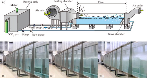
Wind velocity was measured at x=6.5 m by using both a laser Doppler anemometer and a phase Doppler anemometer (Dantec LDA, PDA). Air-friction velocity u* was estimated by an eddy correlation method on the air side. Wind speed at z=10 m height U ₁₀ was estimated from the log law in airflow. Water-level fluctuation was measured with resistance-type wave gauges (Kenek CHT4-HR60BNC) at x=6.5 m. The average water level was measured with a resistance-type water-level gauge (Kenek CWT-20KWT) connected by tubes to the wind-wave tank. The details of the measuring technique are shown in Takagaki et al. (2012).

The mass transfer velocity k _L was estimated by applying a mass balance method for the whole wind-wave tank in CO₂ evasion experiments. This technique is almost the same as used in Ocampo-Torres and Donelan (1994). CO₂ gas was dissolved to excess in fresh water in tanks before evasion experiments. By circulating water between the wind-wave tank and the reserve tank, we maintained an almost homogeneous CO₂ concentration throughout the wind-wave tank. The water volume of the wind-wave tank and the reserve tank were 9.9 and 4.0 m³, respectively. The circulation time ranged from 2 hours at the lowest wind speed to 8 minutes at the highest wind speed. Wind waves were driven in the wind-wave tank by the interfacial shear of wind generated by a fan. The free-stream wind speed U _∞ ranged from 5 to 43 m s⁻¹, where U _∞ in the wind-wave tank is the maximum mean velocity at the outer edge of the air boundary layer above the air–water interface. At extremely high wind speeds, the water volume of the wind-wave tank decreased during the experiments because some amount of dispersing droplets generated by intense wave breaking passed out through the outlet of the tank (Fig. 1a). To compensate for the water loss, the water volume of the tank was kept constant by supplying fresh and uncarbonated water in the upstream region of the tank. The maximum supplied amount of water was 1.83×10⁻³ m³ s⁻¹ at the highest wind speed. Assuming that the CO₂ concentration in the dispersing droplets to be the same as that in the bulk water, the maximum flux of CO₂ discharged by dispersing droplets outside the tank can be estimated to be less than 8% of total CO₂ flux across the wind-driven air–water interface even at the highest wind speed. Therefore, the measurement error was less than 8%.

The CO₂-contained water was sampled via four sampling tubes at x=6.5 m and z=−0.05, −0.25, −0.5, −0.7 m. The concentration of the total dissolved inorganic carbon (DIC) in the sampled water was measured with a total organic carbon meter (TOC-V-CSH, Shimadzu) every 3 minutes. As the ratio of undissociated CO₂ to the DIC depends on pH, the pH in the sampled water was simultaneously measured with a pH meter (F-52, HORIBA). Temperature was measured by a thermo couple (HA-202K, Anritsu Meter) at x=6.5 m and z=−0.4 m. Air was continuously blown over the interface until the CO₂ concentration in the bulk water was decreased by evasion from the hundreds to the tens of mg L⁻¹. Sampling periods ranged from 5 hours at the lowest wind speed to 16 minutes at the highest wind speed. All measurements were conducted at the centre of the tank (y=0).

The mass transfer velocity k _L in eq. (1) was calculated as follows2

where [CO_2aqw] and [CO_2aqi] are the aqueous CO₂ concentration in the bulk water and that at the air–water interface, respectively. When CO₂ is homogeneously mixed throughout the tank, CO₂ flux across the air–water interface F is given as follows:3

where [DIC] is the concentration of DIC in the bulk water, V _w is the total volume of water in both tanks, and A is the area of the wind-wave interface projected onto the x–y plane. The concentration of aqueous CO₂ in clean water which is in equilibrium with the atmosphere (CO₂ concentration in air = 400 ppm) was 0.7 mg L⁻¹ at 20°C. However, [CO_2aqw] in the bulk water was 27–360 mg L⁻¹ during the evasion experiments because we excessively dissolved CO₂ into water before starting experiments. Thus, [CO_2aqi] which is in equilibrium with the atmosphere was less than 3% of [CO_2aqw]. This enabled us to neglect [CO_2aqi] in eq. (3) and therefore k _L was given as follows:4

where Δt is the sampling interval and Δ[DIC] is the change in the concentration of DIC over the Δt. By taking the time average of eq. (4), k _L was calculated and converted into k _L* at 20°C by using the relation between the Schmidt number Sc for CO₂ in water at any temperature and Sc* at 20°C (=600):5

where Sc was calculated from the diffusion coefficient of CO₂ (Yasunishi and Yoshida, 1978). Hereafter, the converted k _L* is denoted as k _L.

3. Results and discussion

3.1. Relationships between mass transfer velocity and wind speeds or air-friction velocity

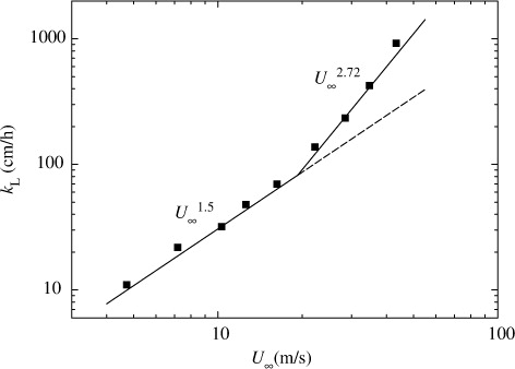
Figures (2–4) show the relationships between mass transfer velocity k _L and three velocities of air-friction velocity u*, wind speed at 10 m height U ₁₀ and free-stream wind speed U _∞. Here, the present U ₁₀ and u* were in good agreement with the empirical relations obtained from the measurements of Takagaki et al. (2012):6 7

Fig. 2 Mass transfer velocity k _L against air-friction velocity u*.

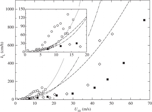
Fig. 3 Mass transfer velocity k _L against wind speed at 10 m height U ₁₀.

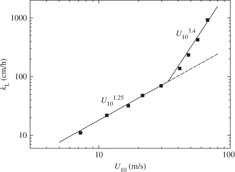
Fig. 4 Mass transfer velocity k _L against free-stream wind speed U _∞.

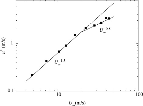
In addition, the relationship between u* and U _∞ in the wind-wave tank was given by following equations from present measurements in Fig. 5:8

Fig. 5 Air-friction velocity u* against free-stream wind speed U _∞.

The mass transfer velocity k _L increases in proportion to u* up to u*~1.7 m s⁻¹ and then much more rapidly in proportion to u*^3.4 at u*≳1.7 m s⁻¹. This pattern suggests that the mechanism of CO₂ transfer changes at u*~1.7 m s⁻¹. The relationships between k _L and U ₁₀ and k _L and U _∞ also show similar increasing tendency to k _L against u* and the relationships between k _L and three wind speeds are given by:9 10 11

At low and moderate wind speeds, CO₂ transfer across the wind-driven air–water interface is promoted mainly by turbulent eddies generated by wind shear stress acting on the air–water interface (Komori et al., 1993). At extremely high wind speeds, however, the interface is intensively broken and wave breaking generates a lot of droplets dispersing in the air and a lot of bubbles in the water (e.g. Zhao et al., 2006). In fact, the volume flux of dispersing droplets lost through the outlet of the tank V _OUT increases drastically at u*≳1.7 m s⁻¹ as shown in Fig. 6. In addition, the increasing rate of u* against U _∞ changes at U _∞≳19 m s⁻¹ (u*≳1.7 m s⁻¹) as shown in Fig. 5. This means that the intensive wave breaking occurs at u*≳1.7 m s⁻¹ as seen in the change of the increasing rate of significant wind waves H _s in Fig. 7 and it affects the flow structure. These results suggest that intense wave breaking has significant effects on CO₂ transfer at extremely high wind speeds. In this experiment, the maximum wavelength of wind waves L in the wind-wave tank was about 1.9 m at the highest wind speed (U _∞=43 m s⁻¹). The water depth D in the tank was set to 0.8 m. Therefore, the ratio of the water depth to the wavelength D/L was nearly 0.5 which is a strict criterion for deep water waves, and the wind waves in our wind-wave tank could be regarded as almost deep water waves under all experimental conditions in this study. This means that the shapes of the wind waves are not affected by the water depth in the wind-wave tank and the amount of the entrained bubbles is not affected by the water depth. However, we could not compare the penetration depths of bubbles between the wind-wave tank and the real oceans because of lack of field data at extremely high wind speeds. Thus, we discussed the dependencies of k _L on wind parameters without going into the problem of the penetration depth.

3.2. Comparison between laboratory and field measurements

Figures 8 and 9 again show the dependencies of k _L on u* and U ₁₀ for present laboratory and previous field experiments. The values of u* in the field measurements were calculated from U ₁₀ by using eqs. (6) and (7). The values of k _L are normalized to Sc=660 (sea water at 20°C). The laboratory measurements of k _L are lower than most field measurements. Only the field measurements of McNeil and D'Asaro (2007) are close to our data, but the validity of their new method has not been well confirmed. One of the reasons of difference between laboratory and most field measurements except McNeil and D'Asaro (2007) might be attributed to the effect of fetch, which is too short in our tank to allow us to investigate its effect on k _L.

Fig. 6 Volume flux of dispersing droplets V _OUT against air-friction velocity u*.

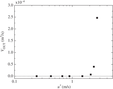
Fig. 7 Mean height of significant waves H _s against air-friction velocity u*.

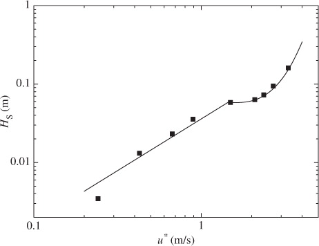
Fig. 8 Comparison of k _L between laboratory and field measurements against u*. Data from this study (laboratory, CO₂, solid squares), McGillis et al. (2001) (field, CO₂, open squares), McGillis et al. (2004) (field, CO₂, open triangles), Jacobs et al. (2002) (field, CO₂, open circles), McNeil and D'Asaro (2007) (field, O₂ and N₂, open diamonds). A dashed line, a dotted line and a dashed-dotted line show the conventional k _L correlation curves proposed by Wanninkhof (1992), Wanninkhof and McGillis (1999) and Wanninkhof et al. (2009) respectively.

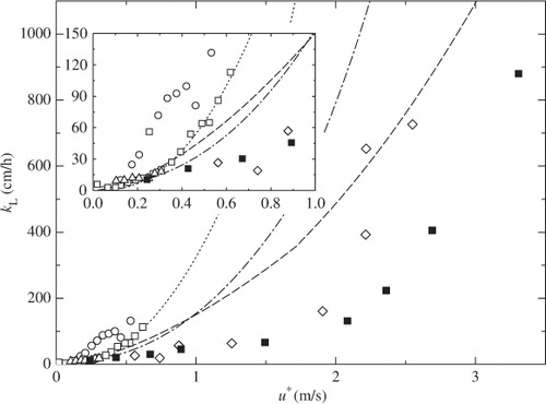
Fig. 9 Comparison of k _L against U ₁₀ between laboratory and field measurements. Symbols and lines as in Fig. 8.

On the other hand, Komori (2013) found that k _L is well correlated with the free-stream wind speed U _∞ independent of the fetch. Komori et al. (1982) also suggested a strong correlation between k _L and U _∞. Figure 10 again shows the relationship between k _L and U _∞ for present laboratory and previous field experiments and the correlation curve of eq. (11) normalized to Sc=660 is also indicated by a solid line in the figure. Here, the free-stream wind speed U _∞ at the outer edge of the atmospheric boundary layer above the air–sea interface was approximately given by the wind speed estimated on the basis of the log law at the height of 65 m above the air–sea interface U ₆₅ (Jones and Toba, 2001; Komori, 2013). From the log law together with eq. (7), the free-stream wind speed is given by:12

Fig. 10 Comparison of k _L against U _∞ between laboratory and field measurements. Symbols and lines as in Fig. 8. A solid line shows the correlation curve of eq. (11) normalized to Sc=660 for the present laboratory measurements.

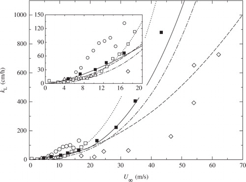
When U _∞ is given by eq. (12), both laboratory and field measurements of k _L are well correlated with U _∞ at U _∞≲19 m s⁻¹. The present values of k _L closely approximated the conventional correlation curves of Wanninkhof (1992), Wanninkhof and McGillis (1999) and Wanninkhof et al. (2009) at the low and moderate wind speeds of U _∞≲19 m s⁻¹ when U _∞ replaces U ₁₀ in their correlation curves. However, at extremely high wind speeds of U _∞≳19 m s⁻¹, the present data deviate from the correlation curves of Wanninkhof (1992) and Wanninkhof and McGillis (1999) and approach that of Wanninkhof et al. (2009) as wind speed increases. This indicates that mass transfer is greatly enhanced by the intense wave breaking at extremely high wind speeds, and the correlation curve of Wanninkhof et al. (2009) is appropriate for the correlation between k _L and U _∞ for wide range including extremely high free-stream wind speeds. This would be because that Wanninkhof et al. (2009) expressed k _L as a third-order polynomial function of wind speed which can capture multiple processes that control mass transfer such as wave breaking, whereas Wanninkhof (1992) and Wanninkhof and McGillis (1999) assume a simple quadratic or cubic dependency.

4. Conclusions

Mass transfer velocity k _L increases drastically at extremely high wind speeds of u*≳1.7 m s⁻¹, U ₁₀≳34 m s⁻¹ and U _∞≳19 m s⁻¹. The volume flux of dispersing droplets begins to increase drastically and the mean height of significant waves also changes its rate of increase at almost the same wind speed as that at which the rate of increase of k _L changes. This change indicates that intense wave breaking occurs at extremely high wind speeds and it has significant effects on CO₂ transfer. At low and moderate wind speeds, laboratory and field measurements of k _L are well correlated with the free-stream wind speed and the present values of k _L closely approximate the conventional correlation curves of Wanninkhof (1992), Wanninkhof and McGillis (1999) and Wanninkhof et al. (2009) when U _∞ replaces U ₁₀ in their correlation curves. However, at extremely high wind speeds, the present data deviate upward from the correlation curves of Wanninkhof (1992) and Wanninkhof and McGillis (1999) and approach to that of Wanninkhof et al. (2009) as wind speed increases. This indicates that the correlation curve of Wanninkhof et al. (2009) better represents the correlation between k _L and U _∞ for extremely high free-stream wind speeds than curves of Wanninkhof (1992) and Wanninkhof and McGillis (1999).

Acknowledgements

This work was supported by the Ministry of Education, Culture, Sports, Science and Technology, Grant-in-Aid (25249013, 24360069 and 23-1490). The authors also thank H. Kamiuchi and M. Nishihira for their help in conducting experiments.

Notes

A Erratum has been published for this paper. Please see http://www.tellusb.net/index.php/tellusb/article/view/25233

References

- Bates N. R , Knap A. H , Michaels A. F . Contribution of hurricanes to local and global estimates of air–sea exchange of CO2 . Nature. 1998; 395: 58–61.
- Hare J. E , Fairall C. W , McGillis W. R , Edson J. B , Ward B , co-authors . Evaluation of the National Oceanic and Atmospheric Administration/Coupled-Ocean Atmospheric Response Experiment (NOAA/COARE) air–sea gas transfer parameterization using GasEx data. J. Geophys. Res. 2004; 109: 08S11. 10.1029/2003JC001831.
- Jacobs C , Kjeld J. F , Nightingale P , Upstill-Goddard R , Larsen S , co-authors . Possible errors in CO2 air–sea transfer velocity from deliberate tracer releases and eddy covariance measurements due to near-surface concentration gradients. J. Geophys. Res. 2002; 107(C9): 3128. 10.1029/2001JC000983.
- Jones I. S. F , Toba Y . Wind Stress Over the Ocean. 2013; Boca Raton: CRC Press. 479–488. Vol. 1 .
- Koch J. , McKinley G. A. , Bennington V. , Ullman D . Do hurricanes cause significant interannual variability in the air–sea CO2 flux of the subtropical North Atlantic?. Geophys. Res. Lett. 2009; 36: 07606. 10.1029/2009GL037553.
- Komori S . Fernando H. J. S . Turbulent gas transfer across air-water interfaces. Handbook of Environmental Fluid Dynamics. 2013; Boca Raton: CRC Press. 479–488. Vol. 1 .
- Komori S , Nagaosa R , Murakami Y . Turbulence structure and mass transfer across a sheared air–water interface in wind-driven turbulence. J. Fluid. Mech. 1993; 249: 161–183.
- Komori S , Ueda H , Ogino F , Mizushina T . Turbulence structure and transport mechanism at the free surface in an open channel flow. Int. J. Heat Mass. Tran. 1982; 25: 513–521.
- McGillis W. R , Edson J. B , Hare J. E , Fairall C. W . Direct covariance air–sea CO2 fluxes. J. Geophys. Res. 2001; 106(C8): 16729–16745. 10.1029/2000JC000506.
- McGillis W. R , Edson J. B , Zappa C. J , Ware J. D , McKenna S. P , co-authors . Air–sea CO2 exchange in the equatorial Pacific. J. Geophys. Res. 2004; 109: 08S02. 10.1029/2003JC002256.
- McNeil C , D'Asaro E . Parameterization of air-sea gas fluxes at extreme wind speeds. J. Mar. Sys. 2007; 66: 110–121.
- Nemoto K , Midorikawa T , Wada A , Ogawa K , Takatani S , co-authors . Continuous observations of atmospheric and oceanic CO2 using a moored buoy in the East China Sea: variations during the passage of typhoons. Deep-Sea Res. II. 2009; 56: 542–553.
- Ocampo-Torres F. J , Donelan M. A . Laboratory measurements of mass transfer of carbon dioxide and water vapour for smooth and rough flow conditions. Tellus. B. 1994; 46: 16–32.
- Takagaki N , Komori S . Effects of rainfall on mass transfer across the air-water interface. J. Geophys. Res. 2007; 112: 06006. 10.1029/2006JC003752.
- Takagaki N , Komori S , Suzuki N , Iwano K , Kuramoto T , co-authors . Strong correlation between the drag coefficient and the shape of the wind sea spectrum over a broad range of wind speeds. Geophys. Res. Lett. 2012; 39: 23604. 10.1029/2012GL053988.
- Wanninkhof R . Relationship between wind speed and gas exchange over the ocean. J. Geophys. Res. 1992; 97(C5): 7373–7382. 10.1029/92JC00188.
- Wanninkhof R , Asher W. E , Ho D. T , Sweeney C , McGillis W. R . Advances in quantifying air–sea gas exchange and environmental forcing. Annu. Rev. Mar. Sci. 2009; 1: 213–244. 10.1146/annurev.marine.010908.163742.
- Wanninkhof R , McGillis W. R . A cubic relationship between air-sea CO2 exchange and wind speed. Geophys. Res. Lett. 1999; 26: 1889–1892. 10.1029/1999GL900363.
- Yasunishi A , Yoshida F . Diffusivity of carbon dioxide in aqueous solution of electrolytes. Kagaku Kogaku Ronbunshu. 1978; 4: 190–194.
- Zhao D , Toba Y , Sugioka K , Komori S . New sea spray generation function for spume droplets. J. Geophys. Res. 2006; 111: 02007. 10.1029/2005JC002960.