A new evaluation of the uncertainty associated with CDIAC estimates of fossil fuel carbon dioxide emission

Abstract

Three uncertainty assessments associated with the global total of carbon dioxide emitted from fossil fuel use and cement production are presented. Each assessment has its own strengths and weaknesses and none give a full uncertainty assessment of the emission estimates. This approach grew out of the lack of independent measurements at the spatial and temporal scales of interest. Issues of dependent and independent data are considered as well as the temporal and spatial relationships of the data. The result is a multifaceted examination of the uncertainty associated with fossil fuel carbon dioxide emission estimates. The three assessments collectively give a range that spans from 1.0 to 13% (2 σ). Greatly simplifying the assessments give a global fossil fuel carbon dioxide uncertainty value of 8.4% (2 σ). In the largest context presented, the determination of fossil fuel emission uncertainty is important for a better understanding of the global carbon cycle and its implications for the physical, economic and political world.

• climate change
• carbon cycle
• uncertainty analysis

1. Introduction

Uncertainty assessments of carbon dioxide emission estimates from fossil fuel (FFCO₂) consumption are cumbersome. Uncertainty quantification is not conducted herein in the classical sense of making an independent determination of the quantity and then comparing that determination to what is measured, or in this case, reported from a calculation result. Part of this cumbersomeness is due to the mismatch in spatial and temporal scales of independent measurements (i.e. commonly point source and instantaneous) and the FFCO₂ quantities calculated (i.e. commonly national and annual). Adding to the cumbersome nature of the uncertainty assessments are potential spatial and temporal correlations in the FFCO₂ estimates and underlying calculation data; the lack of fully independent FFCO₂ inventory data from other data providers; and while the input inventory data are rich in space and time at the global scale, they are sparse in space and time at the national scale for specific fuels. All of these issues are discussed further in the following text. FFCO₂ uncertainty assessments conducted herein are based on aspects of the calculation for which some measure of uncertainty quantification can be based. Quantification of uncertainty may include expert judgment, statistical sampling, constraints imposed by a larger system of which FFCO₂ is only a part (e.g. the global carbon cycle), or by comparison with other estimates of the same quantity (which may be partially dependent or independent of the original calculation).

Estimates of FFCO₂ have been published by the Carbon Dioxide Information Analysis Center (CDIAC), Oak Ridge National Laboratory (ORNL), United States, since 1984 and are broadly used by scientists, decision makers and civil society. CDIAC FFCO₂ estimates include both national and global totals and extend in annual increments back to 1751. One focus of CDIAC efforts is to provide consistent and reliable FFCO₂ emission estimates on national and global totals across countries and time. Marland and Rotty (1984) published a global total range of uncertainty of 6–10% (90% confidence interval), depending on the independence of the values used in the calculation. CDIAC has never published quantitative values for the uncertainty in national emissions, although many data users are aware that the uncertainty varies widely among countries.

With increasing interest in the magnitude of FFCO₂ emission estimates, the uncertainty surrounding their estimates takes on considerable importance. Uncertainty in FFCO₂ emissions affects the understanding of the global carbon cycle (Bindoff et al., 2007; Denman et al., 2007; Forster et al., 2007; Hegerl et al., 2007; Le Treut et al., 2007; Le Quéré et al., 2009), the design and implementation of mitigation measures, and the ability to monitor and verify mitigation commitments at all levels (e.g. Pacala et al., 2010). National estimates of FFCO₂ emissions from all or most countries are now provided by a number of organisations [e.g. International Energy Agency (http://www.iea.org), the Energy Information Administration of the United States Department of Energy (http://www.eia.doe.gov), and a joint effort of the Joint Research Centre of the European Commission and PBL Netherlands Environmental Assessment Agency (http://edgar.jrc.ec.europa.eu)]. Signatory countries are obligated to report their own estimates of emissions to the United Nations Framework Convention on Climate Change. There have been many efforts to compare various FFCO₂ estimates (e.g. Marland et al., 2007; Macknick, 2009; Afsah and Aller, 2010; Ciais et al., 2010; Andres et al., 2012), but the task is not trivial. Francey et al. (2013) suggest large underreporting, and hence uncertainty, in the global total of FFCO₂ emissions around years 1995–2005 based on atmospheric measurements. This manuscript does not attempt to compare national/global FFCO₂ estimates from different sources, nor does it attempt to evaluate the relative quality of the different sources of FFCO₂ data. The manuscript does suggest that in many cases, the best estimates of current national emissions will be those published by the individual countries wherein they have access to the most-detailed fuel consumption statistics and country-specific coefficients.

In this manuscript, three uncertainty assessments of the CDIAC FFCO₂ emission estimates are presented. All three approach the uncertainty of FFCO₂ estimates by examining the data themselves, but they approach the uncertainty from different aspects. None of the assessments fully evaluate the entire FFCO₂ data set with all of its components. However, each assessment focuses on at least one component. Combined, the three assessments give a multifaceted examination of the uncertainty associated with FFCO₂ emissions.

Many users of FFCO₂ estimates are most concerned with the global total of FFCO₂ emissions. However, the global total is rarely directly calculated. The global total is often the sum of the national totals plus an additional term for emissions that are not included in national totals (e.g. bunker fuels which are fuels used in international trade, Andres et al., 2012). In this manuscript, one uncertainty assessment is based on data at the global level (i.e. the 1-D case) and two uncertainty assessments are based on data at the national level (i.e. the 2-D and 3-D cases).

Adding to the cumbersomeness of the uncertainty quantification presented, FFCO₂ emission estimates do not fit neatly into the categories of dependent or independent data (at nearly all levels of the calculations) for which classical uncertainty quantification approaches are well established. Independence refers to if a particular FFCO₂ emission estimate does not share factors with any other FFCO₂ emission estimate. Dependence refers to if a particular FFCO₂ emission estimate does share factors with another FFCO₂ emission estimate. For example, while the emissions from some countries are calculated with country-specific emission factors (i.e. independent), others are calculated with global default emission factors (i.e. dependent). Even within one country, emissions from one fuel source (e.g. solid, liquid, or gaseous fuels) may be calculated with country-specific emission factors while emissions from another fuel source may rely on global default emission factors. Additionally, it is not a fully compensatory system (i.e. a zero-sum game) where a deficit in emissions from one country is compensated by a surplus in emissions from another country. This non-compensation applies both temporally and spatially. For example, fossil fuels produced in one yr are not necessarily consumed in that same year (i.e. there are changes in stocks from year to year). Also, fuel trading is not perfectly reported (i.e. the sum of fuel imports for all countries does not equal the sum of fuel exports for all countries). Therefore, uncertainty assessments can be calculated with the classical approaches of data dependence or independence, which then act as end-members of the quantification of uncertainty. The true value presumably lies between these end-members.

This end-member approach was the approach originally adopted by Marland and Rotty (1984). The uncertainty assessment of Marland and Rotty (1984) has been often overlooked by the broader community which has often treated the FFCO₂ emission estimates as if they had negligible uncertainty associated with them. This treatment may be due to the relatively small uncertainty associated with the FFCO₂ emission estimates (especially in comparison to other components of the global carbon cycle in either absolute mass or relative percentage units) or to expediency in calculations involving the global carbon cycle (e.g. inverse model calculations which assume the FFCO₂ emissions have zero uncertainty, Gurney et al., 2002). In the almost 30 yr since Marland and Rotty (1984), the environment surrounding FFCO₂ emissions and the global carbon cycle have changed dramatically. The many fluxes and reservoirs in the global carbon cycle and the uncertainties surrounding those fluxes and reservoirs have been better quantified. Models of the full global carbon cycle have greatly improved and uncertainty propagation through those models is an important component to the understanding of the global carbon cycle and any subsequent effects the carbon cycle may have on the physical, economic and political world. It is in this light that this manuscript is written. The objective in this manuscript is to revisit, update and expand on the Marland and Rotty (1984) uncertainty assessment by providing insight on the magnitude and nature of uncertainty in the CDIAC data. The focus remains entirely on the CDIAC emission estimates, but the ideas discussed have broad relevance to other estimates of FFCO₂. This uncertainty assessment was intentionally not applied to other global FFCO₂ emission inventories because as with the CDIAC data, much of the underlying data is not freely available (due to data collection and sharing agreements) and thus the uncertainty analysis applied herein is best applied by providers of those other inventories and not by outside parties who do not have full access to the underlying data.

2. A brief review of CDIAC FFCO₂ emission estimate calculations

For a given country in a given year, the estimate of FFCO₂ emissions is given by1

where FC is the amount of fossil fuel consumed (typically in units of mass, volume, or energy), FO is the fraction of fuel oxidised during combustion or other use (1-FO is the carbon left as durable products such as soot, asphalt or synthetic fabrics), and CC is the carbon content of the fuel (typically in units of tonne C/tonne fuel). The global total of emissions is then given by the summation of this equation over all countries in one yr. For global totals, production data are preferred to consumption data to give the FC used in eq. (1). See Andres et al. (2012) for more details regarding calculations with fuel production and consumption data.

Geographic localisation of the FFCO₂ emission estimates can be given by apparent consumption (AC), where2

summed over all fuel commodities (e.g. natural gas, jet fuel, brown coal coke). See Andres et al. (2012) for more details regarding AC. This AC equation gives the FC used in eq. (1) when calculating non-global totals (e.g. national totals). If AC is used to calculate a global total FFCO₂ emission based on the sum of national emissions, then an additional term is needed to account for fuels not included in national accounts (e.g. bunker fuels).

For FFCO₂ emission estimates produced at CDIAC, FC are largely taken from the United Nations Statistics Division Energy Statistics Database (http://unstats.un.org/unsd/energy/edbase.htm). For the latest release of the database, covering emission years 1950–2010, more than 327 000 individual data points were used. Each data point is labelled by country, year, fuel commodity, units, transaction type (e.g. gross production, import, export) and footnotes. FO are taken from a variety of published and unpublished data and are customised to global averages for each major fuel type (i.e. solid fuels, liquid fuels, gaseous fuels, gas flaring and cement). CC are taken from a variety of published and unpublished data and are customised to global averages for each major fuel type. However, for solid fuels, separate global default averages for CC are used for hard and soft coals. Additionally, because coals have the most variable carbon content of all the fuels and because energy content is better correlated with CC than is mass, countries may and many do provide country and year specific heating values (which are used to convert the United Nations’ reported mass units to energy units and are then related to carbon content, see Marland et al., 2007). For the latest release of the United Nations database, the United Nations reports more than 19 000 individual coal heating values that were subsequently used in the CDIAC FFCO₂ inventory calculations.

CDIAC global and national estimates of FFCO₂ emissions include carbon dioxide emissions from cement production in an effort to produce a more complete accounting of anthropogenic emissions to the atmosphere. Cement production is the largest industrial source of carbon dioxide beyond fossil fuel consumption and comprehensive, worldwide statistics on its production exist (e.g. van Oss, 2013). Cement production releases carbon dioxide when various forms of carbonate are calcined (i.e. heated) to produce clinker (e.g. CaO or MgO). The carbon dioxide released by the calcination process is included in the cement emissions and the carbon dioxide released by the energy used to heat the carbonates is included in the fuel-use emissions. The country where calcination occurs may differ from the country where the resulting oxides are mixed with other ingredients to produce cement. As worldwide statistics tabulate cement production and not clinker production, CDIAC attributes the cement carbon dioxide emissions to the country where the cement was produced, recognising that this should result in a correct estimation of total global emissions from cement manufacture but may attribute some of the national emissions incorrectly (i.e. for clinker that crosses national borders).

The result over time of these emission calculations is a three-dimensional cube of data as seen in Fig. 1. On the front face of the cube, the country names go across the x-axis and the emission years appear along the y-axis. The z-axis is populated by subsequent inventory release years wherein a new emission year of data is added each year and previous emission year data are subject to revision. The front face of the cube contains all of the most recent estimates. The inventory year is equal to the last emission year reported in that inventory plus two; this 2-yr lag reflects the time required for individual national reporting via questionnaire to the United Nations, data collating by the United Nations, and subsequent review and calculation by CDIAC. Elements of the data cube are then populated by the FFCO₂ emission estimates from eq. (1). The AC data, eq. (2), do not appear directly in this cube, but are hidden within the cube calculations and directly affect the FFCO₂ emissions estimates seen in the cube.

Fig. 1 The FFCO₂ emissions estimate data cube. Countries along the x-axis could be labelled by name or number. Emission years used in this analysis range from 1950 to 2010. Inventory years used in the analysis range from 1984 to 2012. Each new release of the CDIAC FFCO₂ inventory adds a new face to the data cube, displacing the old face toward the rear. Not all elements in the data cube are necessarily occupied by valid data. For example, country number 461 could represent Sabah which only has FFCO₂ estimates for emission years 1950–1969. Data elements, for other emission years for this country regardless of the inventory year, are empty since this political unit did not exist in these other emission years. The cube could be filled with emission estimates based on production data only [using eq. (1)] or with emission estimates based on consumption data [additionally using eq. (2)]. The global total FFCO₂ emissions for one emission year in one inventory year could be represented by a horizontal line on the face of the data cube (i.e. the sum of countries). If the cube is filled by consumption data, the global total would require an additional term for emissions that are not included in national totals (e.g. bunker fuels, Andres et al., 2012). For the latest release of the database, more than 107 000 elements of the production data cube are filled and more than 179 000 elements of the consumption data cube are filled. The three insets show which portion of the data cube are used for the 1-D, 2-D and 3-D cases.

Evaluation of the uncertainty associated with the FFCO₂ emission estimates will examine the one- (1-D), two- (2-D) and three-dimensional (3-D) nature of this data cube. Each uncertainty assessment tests some aspects of the data cube more strongly than other assessments.

Two sigma (2 σ) uncertainties are used throughout this manuscript, except where noted. The ±2 σ interval is equal to the 95% confidence interval around the central estimate. This interval was chosen to more strongly convey the message of the probable range of FFCO₂ emissions. Additionally, uncertainties are generally reported to two significant digits, the limit of their precision and accuracy. Finally, anecdotal accounts and some reports (e.g. Environment Canada, 2005; US EPA 2005; US GAO, 2010; Zahar, 2010) suggest symmetry of uncertainty about the central estimate may be incorrect at specific spatial and temporal scales. But, this information is not unidirectional, favouring underestimation or overestimation of FFCO₂, and may have shifted bias in specific times and locales. Therefore, uncertainties in this manuscript are assumed to be symmetric about the central estimate since more detailed information on the extent of asymmetric uncertainties is lacking.

3. Uncertainty assessment: the 1-D case

The 1-D case presented here is a revisit, update and expansion of the Marland and Rotty (1984) uncertainty calculation. This approach examines the terms of eq. (1) for global totals of each fuel separately. There is no national-level uncertainty data in this case. The result is an uncertainty assessment of the global total FFCO₂ emissions estimate that is commonly perceived as time independent. The strength of this approach is that it examines the entire FFCO₂ emissions data set as calculated by fuel production data, as well as continuation of the historical precedent set in Marland and Rotty (1984). The weakness of this approach is that it is more a measure of the global FFCO₂ emission inventory methodology than of the quality of data coming from each country. This approach is equivalent to examining one horizontal stripe on the face of the data cube condensed into one number by summing all of the emissions for a given emission and inventory year.

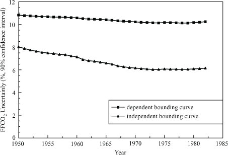
The Marland and Rotty (1984) uncertainty calculation is commonly perceived as a fixed range of 6–10% (90% confidence interval) with the range being defined by independent or dependent uncertainties. That perception is probably based on those are the only values Marland and Rotty (1984) presented and summarised in their conclusions. However, their development of this uncertainty assessment included a time-dependent element in the form of the percentage of each fuel consumed per year. Figure 2 reconstructs the original Marland and Rotty (1984) calculation using their original values and explicitly shows the time trend in their analysis as well as the emission year 1980 points which led to the fixed perception of that analysis. Each data point in each line is the result of the 1-D analysis. The 6% lower bound, based on an independent interpretation of the data, while accurate for emission year 1980 does not characterise well the full time series which initially decreases and then flattens and averages 6.7% (90% confidence interval). The 10% upper bound, based on a dependent interpretation of the data, represents well the relatively flat curve and averages 10% (90% confidence interval) over the years shown.

Fig. 2 The bounding uncertainty curves calculated for the 1-D case as would have been originally calculated by Marland and Rotty (1984). Each data point in each line is the result of the 1-D analysis. Values in the dependent bounding curve were calculated from ∑(f _i *combined_i) and values in the independent bounding curves were calculated from √∑(f _i *combined_i)², where i=solid fuels, liquid fuels, gas fuels, gas flaring and cement; f is the fraction of the global source in a given year, and combined is from the Table 1 values. Note the 90% confidence interval (1.64 σ) is different than the 2 σ uncertainty assessment used throughout the rest of this manuscript.

In general, for the new analysis reported here, the approach used in the Marland and Rotty (1984) analysis is retained, except for four improvements:

1. Updated uncertainties for the CC component of the calculation as noted in the Table 1 caption

2. Added uncertainty due to the inclusion of cement production [which was not included in the original Marland and Rotty (1984) calculation]

3. Conversion of values from the Marland and Rotty (1984) 90% confidence interval (1.64 σ) to the 2 σ confidence interval used herein

4. Explicitly showing the time trend in the original Marland and Rotty (1984) analysis.

Table 1. Uncertainty data pertinent to the 1-D case

Source	FC (%)	FO (%)	CC (%)	Combined (%)
Solid fuels	14	2.4	4.3	14
Liquid fuels	9.7	3.6	2.2	11
Gas fuels	12	1.2	3.0	13
Gas flaring	24	1.2	4.0	25
Cement	20	4.0	11	23

All values shown are at the 2 σ confidence interval and are shown to two significant digits only. Underlined values have been changed since the Marland and Rotty (1984) calculation. The solid CC uncertainty is new and is based on data reported in Marland et al. (1995), with a fixed coal: lignite ratio of 84: 16 informed by statistics from the entire 1950 to 2010 time series, n=2126. The liquid CC uncertainty is new and is based on data reported by Mash et al. (1995), n=29. The gas CC uncertainty is new and is based on data reported by Liss et al. (1992), n>6800. The gas flaring CC uncertainty is as reported in Boden et al. (1995). Cement uncertainties are discussed in the text. The combined column is the square root of the sum of the squares of FC, FO and CC and indicates the uncertainty for each source. Values shown below are held constant for all years. n=number of samples.

Table 1 does not include updated values for FC and FO for four sources. While independent data exists at the national scale, it is not comprehensive enough in spatial and temporal dimensions to significantly effect the global values originally reported in Marland and Rotty (1984), however, this information can and does get incorporated into the 2-D case described next.

The uncertainty terms for cement are similar to those used for fossil fuels, but have been modified to reflect the cement case. The FC uncertainty of 20% reflects global clinker production knowledge (IPCC, 2006). The FO uncertainty is assumed to be 4% since the calcination zone reaction liberating carbon dioxide is usually driven to completion (Griffin, 1987). The CC uncertainty is 11% as global CaO contents in clinker have some variability (IPCC, 2006). The overall cement uncertainty, 23%, is higher than the 7% determined by the US EPA (2013) for cement carbon dioxide emissions from the United States and is reflective of the wider variety of materials and processes at the global level.

The updated CC components and cement uncertainties reflect new data obtained since Marland and Rotty (1984) was published. These updates cause an increase in uncertainty from 6.1 to 10.2% as originally reported in Marland and Rotty (1984) to 6.1 to 10.5% (using the same 90% confidence interval). The change in confidence interval to 2 σ for emission year 1980 increases the magnitude range of the uncertainty reported to 7.4 to 12.8%.

Figure 3 shows the new 1-D calculation with all CC updates, cement uncertainties and at 2 σ uncertainty. Each data point in each line is the result of the 1-D analysis. The two bounding curves bracket the uncertainty; further quantification of the uncertainty is not easily done in this 1-D assessment. Figure 3 also explicitly shows the time dependency of the calculation. The time-dependent change in uncertainty reflects the changing mix in fuels produced and the different combined fuel uncertainty (see Table 1). For example, the decline in uncertainty early in the time series is driven by decreases in coal consumption relative to liquid fuels and the subtle rise in uncertainty since the year 2000 is due to increasing contributions from coal and cement relative to liquid fuels. For emission year 1980, the revised values are within 0.5% of the original Marland and Rotty (1984) values at the same 90% confidence interval. This implies that this new evaluation of the 1-D case is incremental despite the more complete nature of the new evaluation.

Fig. 3 The bounding uncertainty curves calculated for the 1-D case with all CC updates, cement uncertainties, and at 2 σ uncertainty. The true uncertainty value presumably lies between these bounding curves. Each data point in each line is the result of the 1-D analysis. Note the change in scales from Fig. 2 for both axes to accommodate increased uncertainty magnitude and additional years.

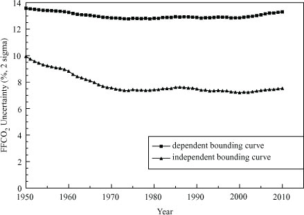
The 3–6% difference between the dependent and independent uncertainty curves, and the large number of emission and inventory years, indicate further analysis may reveal more insights into the nature of the uncertainty surrounding global FFCO₂ emissions. This leads to the 2-D and 3-D case studies.

4. Uncertainty assessment: the 2-D case

The 2-D case presented here is a new approach to uncertainty assessments of FFCO₂ emission estimates. This approach examines global uncertainty as the combination of the uncertainties associated with FFCO₂ emissions from individual countries. Whereas the 1-D case is based on the data for individual fuels, the 2-D case is based on the data for individual countries. Both the 1-D and 2-D cases treat data as dependent or independent. Both the 1-D and 2-D cases result in an uncertainty assessment of the global total FFCO₂ emissions estimate that is time dependent. The strength of the 2-D approach is this time dependency which results from using AC data for FC combined with individual country quantification of uncertainty for FFCO₂ emissions from each country. The weakness of this approach is that it does not explicitly consider all FFCO₂ emissions as emissions not tallied with a specific country are not explicitly considered (bunker fuels are the largest missing component). This approach utilises the face of the data cube by examining all emission years in a single inventory year.

The key input to the 2-D case is to quantify FFCO₂-emission-estimate uncertainty for each individual country. For the present analysis, these uncertainties are based on the qualitative error classes presented in Andres et al. (1996) where countries of similar perceived uncertainty were grouped together in seven classes. This grouping of countries was based on the expert judgment of the authors and their discussions with others knowledgeable about national energy data and FFCO₂ emission estimates. This grouping of countries was a function of both the national energy infrastructure and the national institutions for the collection and management of data related to the flows of energy through that infrastructure. For the present analysis, the seven qualitative classes were quantified by anchoring class 1 (including the United States) and class 6 (including China) with the 2 σ uncertainty assessments presented in Gregg et al. (2008) and then performing a linear interpolation through the other five classes. Table 2 lists the seven classes, the largest FFCO₂ emitter in each class and the associated uncertainty values. To reiterate, the focus in the 2-D case is on data quality by country; the 2-D case reduces the scale from global to national and allows a more customised uncertainty assessment based on national considerations. While uncertainty quantification used in the 2-D case could be improved, the 2-D case leads to interesting and new conclusions discussed below.

Table 2. Uncertainty values pertinent to the 2-D case

Class	Largest FFCO2 emitter	2 σ Uncertainty (%)
1	United States	4.0
2	France	6.7
3	Iran	9.4
4	India	12.1
5	USSR	14.8
6	China	17.5
7	Mexico	20.2

As discussed in the text, these values are applied for all years. The largest FFCO₂ emitter listed for each class is based on FFCO₂ emission estimates for emission year 1990, the latest emission year available when the classes were first defined. The top emitters in each class are largely the same today with the latest inventory and emission year data, except that class 5 is now led by Russia which is only one of the current national entities that composed the former USSR.

With the given national uncertainty values (σ _i ) and the national masses of FFCO₂ emissions [m _i , using AC data as determined by eq. (2) for FC in eq. (1)], the global uncertainty is determined by the classical approach of3

where i is each individual nation up to a maximum value n (where nations are represented by numerical names instead of text names, see the x-axis of Fig. 1), j equals all nations greater than i until n, and ρ is the correlation of uncertainties between nations (Rencher, 2002). At ρ=0, the second term equals zero, and the uncertainty bounding model of complete data independence is calculated. At ρ=1, the second term has non-zero value, and the uncertainty bounding model of complete data dependence is calculated. The second summation term is similar structurally to the first summation term except that it focuses on the interaction between nations and the factor of two accommodates the symmetry in off-diagonal terms.

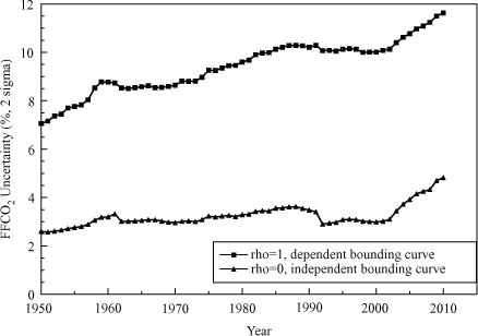
Figure 4 shows the results of eq. (3) used with the latest inventory year data (i.e. for the 1950 to 2010 emission years) and when ρ=0 and ρ=1. The two bounding curves bracket the uncertainty; further quantification of the uncertainty is not easily done in this 2-D assessment. For the completely independent bounding case, 2 σ uncertainty values range over time from 2.6 to 4.8%. For the completely dependent bounding case, 2 σ uncertainty values range over time from 7.1 to 12%. The difference between the two curves ranges over time from 4.5 to 7.2%. The annual values change in response to the changing mass of FFCO₂ emissions associated with each country and its corresponding fixed uncertainty value. In general, the curve values increase in magnitude with time, reflecting a larger mass of FFCO₂ emissions being emitted from countries with larger uncertainties. Although the 2-D case assumption that the uncertainties for each country are fixed over time is likely not valid for all countries, it is also difficult to quantify the extent to which there has been a reduction in national uncertainties as more importance and focus have been attached to national FFCO₂ emission estimates. Decreases in the magnitude of the curve values reflect relatively more emissions being emitted from countries with smaller associated uncertainties; the most prominent example of this is in the lower, independent bounding curve in emission year 1992 where the decrease in magnitude is related to the lowering of emissions from the USSR and eastern Europe due to changes in their political and economic frameworks.

Fig. 4 The bounding uncertainty curves calculated for the 2-D case. Two-sigma uncertainty assessments are calculated for emission years 1950–2010. A better model of uncertainty lies between the two curves shown.

This 2-D approach can be extended to include all FFCO₂ emissions, including those emissions not explicitly incorporated into national emission estimates (such as emissions from bunker fuels). This is done by adding an additional mass term to the calculation which represents this missing mass. However, since the 2-D approach does not reveal substantial information about the uncertainty of this missing mass, it is assigned an uncertainty equal to the global uncertainty calculated by eq. (3). The addition of the magnitude of the missing mass and its uncertainty results in no substantial change to the curves shown in Fig. 4.

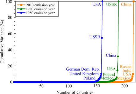
One piece of interesting information that can be derived from eq. (3) in the independent case is a measure of the contribution of each country to the total global uncertainty. This is done by examining the mass weighted variance of each nation (i.e. ) to the total mass-weighted variance. Figure 5 shows a cumulative curve of the contribution to the global variance (uncertainty) from the various nations for the latest inventory year. Only a few countries dominate the variance and thus the uncertainty in a given emission year. This is due to the combination of their relatively large mass of emissions as well as the relative uncertainty associated with those emissions. For example, for emission year 2010, the 200 least-variance-contributing countries sum to only 0.61% of global total variance (uncertainty). China, Russia, India, the United States and Mexico contribute 90, 2.8, 2.5, 2.0 and 0.34%, respectively, to the total global variance and thus 98% of the total global variance is contributed by the FFCO₂ emission estimates of only five countries. This information suggests that in a world of finite resources, the uncertainty in the global total of FFCO₂ emissions could be substantially reduced by focusing effort on only a small number of countries. Clearly the nations labelled at the top of Fig. 5 would be places to concentrate resources. Pacala et al. (2010) made a similar conclusion, but in a more generic sense. This analysis of the contributions to the variance also suggests that if concern is with the reduction of global FFCO₂ emissions uncertainty, than the selection of values for uncertainty of individual countries is not overly important, except for those countries with large emissions or large uncertainty.

Fig. 5 The cumulative variance versus number of nations curve shows the contribution of each nation to total uncertainty. The top five FFCO₂ emitting nations in each emission year are labelled. Some labels could not be clearly placed next to their adjacent data points, but are in the correct top to bottom order. Not all years have the same number of nations. Most nations contribute little to the total variance. All data are from the latest available inventory year.

The 2-D approach could be improved by replacing the linear fit used to quantify uncertainty classes (i.e. Table 2) with individual uncertainty assessments for the 248 individual countries in the CDIAC FFCO₂ database. For the present analysis, this was not done as sufficient independent data for all 248 countries are not available (for the ad hoc and limited collection of independent national emission estimates obtained by the authors, the independent estimate is within the CDIAC national estimate ± linear extrapolated 2 σ). Therefore, the relative groupings and anchored linear extrapolation were employed in this analysis.

The 2-D approach could also be improved by utilising time-varying uncertainty assessments for each country. The time-varying assessments would be a reflection of increased data accuracy due to better estimates of FC, FO and CC due to the improved statistical infrastructure which supports these emission estimates. This improvement will be partially investigated in the next section.

5. Uncertainty assessment: the 3-D case

The 3-D case presented here is a relatively unexplored approach to uncertainty assessments of FFCO₂ emission estimates. Hamal did some initial exploratory research in this area with a much more limited data set than used here and focused mainly on national emission estimates, not global total emission estimates (Marland et al., 2009; Hamal, 2010). Smith et al. (2011) explored a similar approach for anthropogenic sulphur emissions. This approach allows an analysis of how much the current global FFCO₂ total estimate will likely change as a result of future FFCO₂ inventory releases. This approach results in a time dependent uncertainty assessment of the global total FFCO₂ emissions estimate. The strength of this approach is a time-dependency which incorporates not only FC (and AC) changes, but also changes in the basic calculation methodology that CDIAC employs (including changes to FO and CC). FC (and AC) changes mostly reflect revisions and gap filling in the basic energy data sets over time. CDIAC methodological changes over time have been minimal and incremental, but have had a non-zero effect on some FFCO₂ emission estimates. These methodological changes reflect a refinement of the coefficients used in the FFCO₂ emission estimate calculations. The weakness of this approach is that it does not explicitly consider independent information in the determination of uncertainties such as those examined in the 1-D and 2-D cases. This approach utilises the entire data cube by examining all emission years in all inventory years.

The key input to the 3-D case is the collation of data from 21 inventory years into one database; this has not been achieved before. To examine the uncertainty associated with the latest estimate of global FFCO₂ emissions, past estimates of global FFCO₂ emissions are examined for how their magnitude has changed with subsequent FFCO₂ inventory releases (i.e. subsequent inventory years) for a given emission year. With this analysis, an attempt to quantify how much the current estimate of FFCO₂ emissions might change in the future is addressed. The 3-D case is based on the assumption that each new inventory year represents the best and most complete data for each emission year [including revisions for FC, FO and CC in eq. (1)], resulting in decreasing uncertainty with each successive revision. Often, much of the input data, especially FC data, are never revisited after the initial compilation and most revisions occur in the first year or first few years after initial reporting.

For this analysis, fuel production data are used for FC in eq. (1) in the calculation of global totals. Production data are believed to have lower uncertainty associated with them than AC data as explained in Andres et al., 2012. Production data have the advantage of no ‘leakage’ associated with them (e.g. temporally via changes in stocks or spatially via imports/exports and bunker fuels), but have the disadvantage of lacking local specificity in emissions (i.e. at the national level). For the global focus of this analysis, this disadvantage is not important. For the other terms of eq. (1), FO and CC, changed values were incorporated into this analysis as they were changed in the historical development of the CDIAC database.

To examine how global FFCO₂ emission estimates change in subsequent inventory years, the earliest inventory year in which an emission year global FFCO₂ emission estimate occurs is taken as the baseline estimate. This baseline estimate is then used as the comparator to calculate difference and per cent differences with subsequent inventory years for a given emission year.

Figure 6 shows the magnitude of the difference between initially estimated global FFCO₂ emission estimates and each subsequent revision thereof with subsequent inventory years. Negative values indicate the first inventory year was larger than a subsequent inventory year for a given emission year, positive values indicate the first emission year was smaller than a later inventory year for a given emission year. By definition, the first inventory year of an emission year is equal to zero.

Fig. 6 3-D case: The difference in global FFCO₂ emission estimates as calculated in subsequent inventory years for a given emission year. All curves start at zero by definition. The 61 individual emission years (i.e. 1950–2010) are not individually labelled. The first curve starting at the left of the plot is for emission year 1950 and shows the difference in reported 1950 emissions with each successive reported inventory (i.e. inventory years). Many emission years show an increase in the difference at inventory year 2006 which is discussed in the text.

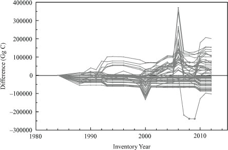
The largest positive difference (370 000 Gg C) is seen for emission year 2000 in inventory year 2006 and that spike is common to all emission years after 1979 (except 2004 which is equal to zero, by definition). This spike is due to two main factors: (1) a 30% revision in Chinese coal production data which accounts for 50% of the spike and (2) a 1-yr change in definitions applied to the United Nations Statistics Division Energy Statistics Database. In this year, the United Nations temporarily characterised a secondary (i.e. derived) fuel as a primary fuel, thus allowing a double counting. The largest negative difference (−240 000 Gg) is seen for emission year 2004 in inventory year 2009 and is also due to two factors: (1) the definition correction mentioned in the last sentence propagates through this emission year (i.e. the comparator is relatively large) and (2) there were significant changes in reported coal production from China, the Russian Federation and Australia. Both the largest positive and largest negative differences highlight the strength of the 3-D uncertainty assessment: changes in FC are coupled with CDIAC methodological changes.

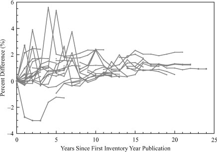
While difference values appear large in magnitude (Fig. 6), relative to the total magnitude of FFCO₂ emission estimates for a given emission year they are small (see Fig. 7 where they appear in per cent difference units). Figure 7 also more directly addresses the analysis question by displacing the curves along the relabelled x-axis so that revisions since the first inventory publication of an emission year are more clearly seen. Only the most recent 25 of the 61 emission year curves are plotted here because older emission years experience two or more inventory years before they are revised, thus eliminating the possibility of seeing shorter term variations. Figure 7 shows that after 10 yr since first publication, global FFCO₂ inventory revisions centre around a 1.1% growth (range 0.28–2.4%) with a standard deviation of 1.0% (2 σ). For the first 10 yr, global FFCO₂ inventory revisions centre around a lower average, 0.74% growth, but have a wider range (−3.0–5.6%) and standard deviation (2.3%, 2 σ). These standard deviations reflect both FC and CDIAC methodological changes. The average increase of global emissions for a given emission year with subsequent inventory years is attributed to more complete reporting as additional data are incorporated into the national reporting. Excluding the spikes in global emissions discussed in relationship to differences (i.e. Fig. 6), the wider range of global emissions for a given emission year in the inventory years following first release is largely attributed to revisions in originally reported energy data.

Fig. 7 3-D case: The per cent difference in global FFCO₂ emission estimates as calculated in subsequent inventory years for a given emission year. All curves start at zero by definition. The 25 individual emission years are not individually labelled.

The assertion that global FFCO₂ totals calculated with production data have lower uncertainty associated with them than those calculated with consumption data can now be tested. In an identical analysis that was done to produce Fig. 7, but completed with consumption data, the results showed an increase from the production-based results discussed in the paragraph above in 2 σ uncertainties for the first 10 yr (3.0%) and after 10 yr (2.6%). Similar in relative magnitude, the uncertainty assessments associated with Fig. 7 (3-D case) are lower in magnitude than those presented in Fig. 4 (2-D case). Both of these examples are consistent with the assertion that global FFCO₂ totals calculated with production data have lower uncertainties associated with them than global FFCO₂ totals calculated with AC data.

6. Underlying data: what are the magnitudes of revisions to national historical FFCO₂ data?

While a departure from the global focus of this manuscript, it follows naturally to discuss briefly the uncertainty in national emissions in a manner similar to the 3-D global uncertainty just described. To examine how national FFCO₂ emission estimates change in subsequent inventory years, the last inventory year in which an emission year national FFCO₂ emission estimate occurs is taken as the baseline estimate. This baseline estimate is then used as the comparator to calculate difference and per cent differences with previous inventory years for a given emission year. As opposed to the previous analysis which used the first reported inventory to determine how much a FFCO₂ emission estimate would change in the future, this analysis uses the last reported inventory based on the assumption that subsequent inventories are more accurate because improved FC data (via additions, deletions and/or corrections) and methodology are employed in its calculation. For this analysis, AC data are used for FC in eq. (1).

Figure 8 shows the minimum and maximum changes for all countries in the CDIAC FFCO₂ database. For example, the United States values (6, −6) show that for all previous inventory years, the maximum upward revision for a given emission year has been 6% from a previously reported inventory year to the currently reported inventory year. Similarly, the maximum downward revision for a given emission year has been −6% from a previously reported inventory year to the currently reported inventory year. The range of emission estimate changes is given in this figure to emphasise the most extreme revisions. Average change and the standard deviation of changes are not given here because, at the national level, those descriptors are often a function of how many revisions have been made rather than the significance of the changes made. For some countries and years, United Nations-collected data are never revised from the initially reported values, and thus their range is (0, 0).

Fig. 8 Maximum and minimum range of per cent change in national emissions for a given emission year. Countries arranged by minimum changes. The group of countries at −100% are countries who had negative calculated emissions that were changed to near zero for this analysis. Eleven countries exceed 400% changes, from left to right (with maximum per cent in parentheses): Netherlands Antilles (2647), Congo (750), Somalia (14217), Gabon (1886), Cape Verde (540), United Arab Emirates (2952), Oman (2191), Côte d'Ivoire (734), Cook Islands (2714), Sierra Leone (2958) and Antarctic Fisheries (7176). Some countries are specifically labelled (with range in parentheses).

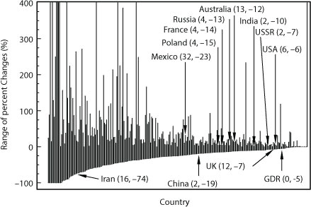
The −100% values seen in Fig. 8 are due to negative national emissions being set to near-zero for this analysis. Thus, when they are revised later, the per cent difference is near −100%. Negative emissions are a statistical construct and usually occur when two large numbers are subtracted from each other [e.g. production and exports, see eq. (2)]. Note that each of these example transactions (i.e. production and exports) have uncertainty associated with them that are not individually evaluated in this manuscript. These countries with negative emissions are followed in Fig. 8 by others who exhibit a similar mathematical path (i.e. a relatively low reported emission estimate is subsequently revised to a higher emission estimate) and whose data are not affected by negative values. The zero minimum per cent difference values reflect that no significant revisions have been made; this may be caused by initially reported values were correct or that the emission year data were not revised in subsequent inventory years.

The large positive maximum values clipped in Fig. 8 result from emission estimates being revised downwards in subsequent years. Thus, the small comparator leads to large per cent differences. The zero maximum per cent difference values reflect that no significant revisions have been made; this may be caused by initially reported values being correct or that the emission year data were not revised in subsequent inventory years.

In addition to giving the range of emission year revisions for all nations, the point of this section is that while major and minor revisions have occurred at the national scale in both increasing and decreasing national FFCO₂ emissions, their cumulative effect at the global scale is generally small (e.g. Fig. 7). However, large revisions in the FFCO₂ emissions data for large FFCO₂-emitting countries do make noticeable changes in the global total FFCO₂ emission estimates, and associated national FFCO₂ uncertainties impact the global uncertainty assessment accordingly (e.g. Fig. 5). For example, if the largest FFCO₂ emitter in emission year 2010, China, were to revise its 2010 emissions downward in a future inventory year by a magnitude equal to its largest magnitude seen previously, −19%, then its corresponding fraction of global total emission would fall from 25 to 21% and the 2-D case uncertainty would fall from the range of 4.8–12% to 4.2–11%.

7. Putting it all together

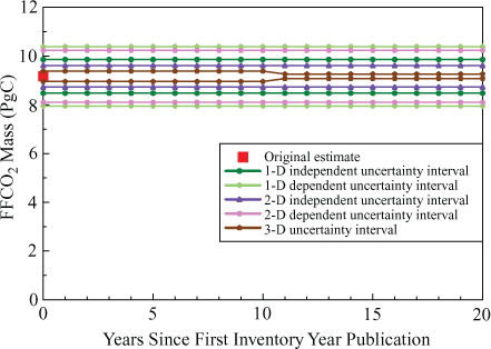
Returning to the global focus of this manuscript, one can envision a 3-D cloud of uncertainty being placed around an emission year global total with the three dimensions being defined by the 1-D, 2-D and 3-D uncertainty cases explored above. However, given the 2-D nature of print media and that two of those dimensions are time invariant for a given emission year, that same information can be represented as shown in Fig. 9. Now, one can clearly see not only the magnitude of FFCO₂ emissions, but also their 95% confidence interval explicitly shown. This figure fulfils the objective of this manuscript as stated in the introduction. Note that the details in this figure will change as different emission years are plotted since the values of the 1-D and 2-D intervals change with emission year.

Fig. 9 Emission year 2010 global FFCO₂ emissions with uncertainties explicitly shown based on the 1-D, 2-D and 3-D uncertainty cases. The time dependent 1-D and 2-D uncertainty cases plot as fixed values for this emission year.

To put this FFCO₂ uncertainty into perspective, it is compared to the uncertainty in other major components in the global carbon cycle in Fig. 10. The components shown in Fig. 10 are simplified by combining many subcomponent fluxes and reservoir stock changes into broad categories. In addition to other carbon cycle components, Fig. 10b, c and d display both the largest (i.e. 1-D dependent) and smallest (i.e. 3-D) uncertainty intervals shown in Fig. 9. This brackets the importance of determining the FFCO₂ uncertainty.

Fig. 10 FFCO₂ compared to other global carbon cycle components. (a) GCP-reported mass flux and reservoir stock changes. Fossil fuels and land use change sources to the atmosphere are balanced by the sinks of atmospheric growth and oceanic uptake with the residual being accommodated by the terrestrial biosphere. (b) Component mass equivalent to 1 σ uncertainty. (c) One σ uncertainty, expressed in per cent of component mass. Terrestrial biosphere flux not shown as described in text. (d) One σ uncertainty, expressed in per cent of total carbon cycle flux and reservoir stock changes. Legend shown is applicable to panels b, c and d.

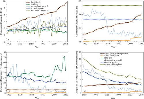
Figure 10a shows the fluxes and reservoir stock changes of the various carbon cycle components as reported by the Global Carbon Project (GCP, http://dx.doi.org/10.3334/CDIAC/GCP_V2012). The FFCO₂ flux initially starts out similar in magnitude to the other components, but grows to be the largest component by the end of the reporting period.

Figure 10b shows the 1 σ uncertainty for the components, expressed in mass units. Uncertainties for the non-FFCO₂ components were reported by the GCP. For the FFCO₂ fluxes, data from this manuscript replaced the GCP-reported values. Regardless of the FFCO₂ uncertainty case used, FFCO₂ has the smallest mass uncertainty shown at the beginning of the reporting period. Dependent on the case used, FFCO₂ ends the reporting period with either the smallest or second largest mass uncertainty. The land use curve lies directly under the oceanic uptake curve. The atmospheric growth rate mass uncertainty drops around 1980 due to a change in how NOAA calculated the uncertainty (http://www.esrl.noaa.gov/gmd/ccgg/trends/global.html).

Figure 10c shows the 1 σ uncertainty for the components, expressed in units of per cent of the component (i.e. Fig. 10b divided by Fig. 10a). Regardless of the FFCO₂ uncertainty case used, FFCO₂ has the smallest per cent uncertainty shown at the beginning of the reporting period. FFCO₂ ends the reporting period with a similar per cent uncertainty to the atmospheric growth rate. Land use change and oceanic uptake have relatively large per cent uncertainties; this suggests potential research opportunities in order to lower these two uncertainties, but the nature of the sampling strategy to reduce these uncertainties is a daunting task. The terrestrial biosphere is not shown in this panel as its range of per cent uncertainty is −620 to 230% which would compress the other components on this panel to overlapping and indistinguishable lines at this scale.

Figure 10d shows the 1 σ uncertain component mass as a percentage of total component mass [i.e. 100*Fig. 10b/(the sum of the five components shown in Fig. 10a)]. Regardless of the FFCO₂ uncertainty case used, FFCO₂ has the smallest per cent uncertainty shown at the beginning of the reporting period. Dependent on the case used, FFCO₂ ends the reporting period with either the smallest (similar to the atmospheric growth rate value) or second largest per cent uncertainty. The land use curve lies directly under the oceanic uptake curve. The general downward trend of the non-FFCO₂ curves as compared to similar curves in Fig. 10c is due to the relatively quicker growing FFCO₂ flux.

8. Conclusions

The CDIAC annual FFCO₂ emission inventories began in 1984 when national and international interest in FFCO₂ emissions was mainly limited to the scientific community and the commitment to collect and analyse energy data was more limited than now. Increasing national and international focus on energy supplies was prompted by the oil crises of the 1970's and the Framework Convention on Climate Change, which entered into force in 1994, have brought much greater attention to energy and FFCO₂ data and have led to more richness and improved quality of data over time. Greater financial and political focus on the energy and FFCO₂ data and its implications are bringing increased scrutiny and transparency. Thus, not only improving the accuracy of the FFCO₂ inventories is increasingly important, but also improving the characterisation of uncertainty of the FFCO₂ inventories is increasingly important.

Despite its importance, the characterisation of uncertainty on estimates of the global total FFCO₂ emission made from the CDIAC database is still cumbersome. The lack of independent measurements at the spatial and temporal scales of interest complicates the characterisation. The mix of dependent and independent data used in the CDIAC calculations further complicates the determination. The three cases presented above collectively give a range of uncertainty that spans 1.0–13%. However, the end members of this range are not calculated on the same basis and each case measures different aspects of the FFCO₂ data cube (Fig. 1). For example, the 1-D case assesses uncertainty primarily from a fuel-based methodology perspective (Table 1). As the contribution of different fuels to total fuel consumption changes annually, so does the annual global uncertainty change (Fig. 3). The 2-D case assesses uncertainty primarily from a national data quality perspective (Table 2). As the contribution from different countries changes annually, so does the annual global uncertainty change. Global uncertainty has been increasing recently (Fig. 4) because more emissions are coming from countries with less certain data collection and management practices (Fig. 5). The 3-D case assesses uncertainty primarily from a data revision perspective (Fig. 7). As data are revised, missing data are reported and methodology refined, global uncertainty for a given emission year settles to typically less than 2% growth after initial data publication.

This manuscript takes three different but complimentary assessments of the uncertainty in CDIAC estimates of FFCO₂ emissions. None of these assessments give a systematic appraisal of the full uncertainty, but collectively they provide useful insights. Greatly simplifying the assessments contained herein and trying to address the community's need for a single, global FFCO₂ uncertainty value, 8.4% (2 σ) is offered as a reasonable combination of the data in Figs. 3, 4 and 7. Given the current data, this greatly simplified uncertainty value is dynamic and may change in the future as the global mix of fuels being consumed changes and as the distribution of those fuels to different countries changes. The lack of independent measurements may also hide systematic errors not incorporated into the three uncertainty cases analysed. If this uncertainty analysis did not capture all relevant terms, the uncertainty may actually be larger than that reported here.

The more-detailed uncertainty cases analysed could be improved if time dependencies were introduced. These time dependencies might be seen in FC, FO and CC uncertainty values (Table 1, 1-D case); and the national emission uncertainty values (Table 2, 2-D case). Smith et al. (2011) introduce a similar temporal uncertainty into their uncertainty assessment for anthropogenic sulphur emissions. Supporting information to critically and comprehensively evaluate these time dependencies for FFCO₂ is lacking at this time. This shortcoming could be addressed by many more studies (e.g. Bond et al., 2006) to collect the detailed information that could then be synthesised for global application. Additionally, as suggested by Marland and Rotty (1984), these factors may partially offset each other (e.g. FO may be improving generally globally due to technological improvements while the proportion of FC from countries with more uncertainty in their reporting is increasing with time). A similar offset was observed by Smith et al. (2011) for anthropogenic sulphur emissions.

An assessment of the autocorrelation of FC with time (Marland and Rotty, 1984; Ballantyne et al., 2012) has also not been included in this analysis. This autocorrelation can come from two sources. First, the FC data for some fuels for some countries exactly repeat their values in subsequent emission years (this affects 4.3% of the FC data in inventory year 2012); this may result from an initial estimate being retained in later years. Second, in countries with slowly changing infrastructures, the FC used in one year is similar to that used in the previous year as production facilities, delivery systems and demand have remained largely unchanged.

This analysis also indicates where additional resources could be best applied in a resource-limited environment. Clearly Table 1 indicates that improved FC statistics could lower global uncertainties. Furthermore, Fig. 5 indicates which countries should presently receive priority for these FC-uncertainty-reducing measures. This echoes and refines the conclusion made in Pacala et al. (2010).

Marland and Rotty (1984) also offer a lengthy qualitative discussion about uncertainty associated with FFCO₂ emissions. This manuscript complements that work by offering additional quantification of FFCO₂ emission uncertainty, especially at the global level. In some ways the situation remains largely unchanged from 30 yr ago, but in other ways improvements can be seen. The core of FFCO₂ emission estimates is still serviced by a relatively small group of interested persons. However, the scrutiny of this work is increasing globally, leading to improved methodologies; forays into new ways of analysing, representing and using the data; and increases in resources available for these efforts. Discrepancies between various data are more quickly identified than previously, but due to the limited nature of the data the cause for the discrepancies are not so quickly resolved. However, FFCO₂ uncertainty assessments are slowly, but surely, moving from a qualitative nature to one more quantitative. The three uncertainty cases presented herein, have attempted to blend the best of the qualitative and quantitative knowledge currently possessed.

Finally, this analysis gives updated uncertainty assessments for the CDIAC FFCO₂ global estimates. It is anticipated that these uncertainty assessments will have three primary impacts. First, these assessments remind the community that FFCO₂ emissions have a non-zero uncertainty associated with them. Second, that this uncertainty is significant, either in isolation or in relation to other components of the global carbon cycle (Fig. 10). Third, that these uncertainty assessments will be used in the next-generation inverse (and other) models to better understand and constrain the global carbon cycle.

9. Acknowledgements

RJA and TAB were sponsored by US Department of Energy, Office of Science, Biological and Environmental Research (BER) programs and performed at Oak Ridge National Laboratory (ORNL) under US Department of Energy contract DE-AC05-00OR22725 to UT-Battelle, LLC. Since the submitted manuscript has been co-authored by a contractor of the US Government, the US Government retains a nonexclusive, royalty-free license to publish or reproduce the published form of this contribution, or allow others to do so, for US Government purposes. Gregg Marland provided helpful discussions and review during the preparation of this manuscript. Two anonymous reviewers provided helpful reviews of the manuscript.

References

- Afsah S. , Aller M . CO2 discrepancies between top data reporters create a quandary for policy analysis. 2010. Online at: http://www.co2scorecard.org/home/researchitem/17 .
- Andres R. J. , Boden T. A. , Bréon F.-M. , Ciais P. , Davis S. , co-authors . A synthesis of carbon dioxide emissions from fossil fuel combustion. Biogeoscience. 2012; 9: 1845–1871.
- Andres R. J. , Marland G. , Fung I. , Matthews E . A one degree by one degree distribution of carbon dioxide emissions from fossil fuel consumption and cement manufacture, 1950–1990. Global Biogeochem. Cycles. 1996; 10: 419–429. DOI: 10.1029/96GB01523.
- Ballantyne A. P. , Alden C. B. , Miller J. B. , Tans P. P. , White J. W. C . Increase in observed net carbon dioxide uptake by land and oceans during the past 50 years. Nature. 2012; 488: 70–72. [PubMed Abstract] DOI: 10.1038/nature11299.
- Bindoff N. L. , Willebrand J. , Artale V. , Cazenave A. , Gregory J. , co-authors . Solomon S. , Qin D. , Manning M. , Chen Z. , Marquis M. , co-editors . Observations: oceanic climate change and sea level. Climate Change 2007: The Physical Science Basis. 2007; Cambridge, UK: Cambridge University Press. 385–432.
- Boden T. A. , Marland G. , Andres R. J . Estimates of Global, Regional, and National Annual CO2 Emissions From Fossil-Fuel Burning, Hydraulic Cement Production, and Gas Flaring: 1950–1992. DOI: 10.1016/j.atmosenv.2005.12.030.
- Bond T. C. , Wehner B. , Plewka A. , Wiedensohler A. , Heintzenberg J. , co-author . Climate-relevant properties of primary particulate emissions from oil and natural gas combustion. Atmos. Environ. 2006; 40: 3574–3587. DOI: 10.1016/j.atmosenv.2005.12.030.
- Ciais P. , Paris J. D. , Marland G. , Peylin P. , Piao S. L. , co-authors . The European carbon balance. Part 1: fossil fuel emissions. Global Change Biol. 2010; 16: 1395–1408. DOI: 10.1111/j.1365-2486.2009.02098.x.
- Denman K. L. , Brasseur G. , Chidthaisong A. , Ciais P. , Cox P. M. , co-authors . Solomon S. , Qin D. , Manning M. , Chen Z. , Marquis M. , co-editors . Couplings between changes in the climate system and biogeochemistry. Climate Change 2007: The Physical Science Basis. 2007; Cambridge, UK: Cambridge University Press. 499–587.
- Environment Canada. Canada's greenhouse gas inventory: 1990–2003 . National Inventory Report, April 15, 2005.
- Forster P. , Ramaswamy V. , Artaxo P , Berntsen T. , Betts R. , co-authors . Solomon S. , Qin D. , Manning M. , Chen Z. , Marquis M. , co-editors . Changes in atmospheric constituents and in radiative forcing. Climate Change 2007: The Physical Science Basis. 2007; Cambridge, UK: Cambridge University Press. 129–234.
- Francey R. J. , Trudinger C. M. , van der Schoot M. , Law R. M. , Krummel P. B. , co-authors . Atmospheric verification of anthropogenic CO2 emission trends. Nat. Clim. Change. 2013; 3: 520–524. DOI: 10.1038/NCLIMATE1817.
- Gregg J. S. , Andres R. J. , Marland G . China: an emissions pattern of the world leader in CO2 emissions from fossil fuel consumption and cement production. Geophys. Res. Lett. 2008; 35: 08806. DOI: 10.1029/2007GL032887.
- Griffin R. C . CO2 Release from Cement Production. [PubMed Abstract].
- Gurney K. R. , Law R. M. , Denning S. A. , Rayner P. J. , Baker D. , co-authors . Towards robust regional estimates of CO2 sources and sinks using atmospheric transport models. Nature. 2002; 415: 626–630. [PubMed Abstract].
- Hamal K . Reporting GHG Emissions: Change in Uncertainty and its Relevance for Detection of Emissions Changes.
- Hegerl G. C. , Zwiers F. W. , Braconnot P. , Gillett N. P. , Luo Y. , co-authors . Solomon S. , Qin D. , Manning M. , Chen Z. , Marquis M. , co-editors . Understanding and attributing climate change. Climate Change 2007: The Physical Science Basis. 2007; Cambridge, UK: Cambridge University Press. 663–745.
- Intergovernmental Panel on Climate Change (IPCC). 2006 IPCC Guidelines for National Greenhouse Gas Inventories, Volume 3: Industrial Processes and Product Use. 2006; Hayama, Japan: Institute for Global Environmental Strategies. 2.7–2.19.
- Le Quéré C. , Raupach M. R. , Canadell J. G. , Marland G. , Bopp L. , co-authors . Trends in the sources and sinks of carbon dioxide. Nat. Geosci. 2009; 2: 831–836. DOI: 10.1038./NGEO689.
- Le Treut H. , Somerville R. , Cubasch U. , Ding Y. , Mauritzen C. , co-authors . Solomon S. , Qin D. , Manning M. , Chen Z. , Marquis M. , co-editors . Historical overview of climate change. Climate Change 2007: The Physical Science Basis. 2007; Cambridge, UK: Cambridge University Press. 93–127.
- Liss W. E. , Thrasher W. H. , Steinmetz G. F. , Chowdiah P. , Attari A . Variability of Natural Gas Composition in Select Major Metropolitan Areas of the United States.
- Macknick J . Energy and Carbon Dioxide Emission Data Uncertainties. 2009; Laxenburg, Austria: International Institute for Applied Systems Analysis. 55. IR-09-032.
- Marland G. , Andres R J. , Blasing T. J. , Boden T. A. , Broniak C. T. , co-authors . King A. W. , Dilling L. , Zimmerman G. P. , Fairman D. M. , Houghton R. A. , co–editors . Energy, industry and waste management activities: an introduction to CO2 emissions from fossil fuels. The First State of the Carbon Cycle Report (SOCCR): The North American Carbon Budget and Implications for the Global Carbon Cycle. 2007; Asheville, NC: U.S. Climate Change Science Program and the Subcommittee on Global Change Research. 57–64.
- Marland G. , Boden T. , Andres R. J . Carbon dioxide emissions from fossil fuel burning: emissions coefficients and the global contribution of eastern European countries. Idojárás. 1995; 99: 157–170.
- Marland G. , Hamal K. , Jonas M . How uncertain are estimates of CO2 emissions?. J. Ind. Ecol. 2009; 13: 4–7. DOI: 10.1111/j.1530-9290.2009.00108.x.
- Marland G. , Rotty R. M . Carbon dioxide emissions from fossil fuels: a procedure for estimation and results for 1950–1982. Tellus B. 1984; 36: 232–261. DOI: 10.1111/j.1600-0889.1984.tb00245.x.
- Mash H. E. , Andres R. J. , Marland G. , Boden T . Emissions of carbon dioxide from the combustion of fossil fuels. 1995; Programs & Progress, Research Triangle Park, NC, USA: AWMA Meeting on The Emissions Inventory:.
- Pacala S. W. , Breidenich C. , Brewer P. G. , Fung I. , Gunson M. R. , co-authors . Verifying Greenhouse Gas Emissions: Methods to Support International Climate Agreements. DOI: 10.5194/acp-11-1101-2011.
- Rencher A. C . Methods of Multivariate Analysis. 2002; , New York, NY: Wiley.
- Smith S. J. , van Aardenne J. , Klimont Z. , Andres R. J. , Volke A. , co-author . Anthropogenic sulfur dioxide emissions: 1850–2005. Atmos. Chem. Phys. 2011; 11: 1101–1116. DOI: 10.5194/acp-11-1101-2011.
- United States Environmental Protection Agency (US EPA). Inventory of U.S. Greenhouse Gas Emissions and Sinks: 1990–2003.
- United States Environmental Protection Agency (US EPA). Inventory of U.S. Greenhouse Gas Emissions and Sinks: 1990 – 2011. 2013. Online at: http://www.epa.gov/climatechange/Downloads/ghgemissions/US-GHG-Inventory-2013-Main-Text.pdf.
- United States Government Accountability Office (US GAO). Climate Change: The Quality, Comparability, and Review of Emissions Inventories Vary Between Developed and Developing Nations. 2010; DC: Washington.52. GAO-10-818, GAO.
- van Oss H. G . Cement 2011 Minerals Yearbook. 2013; Washington, DC: U. S. Geological Survey. 16.1–16.33.
- Zahar A . Does self-interest skew state reporting of greenhouse gas emissions? A preliminary analysis based on the first verified emissions estimates under the Kyoto protocol. Clim. Law. 2010; 1: 313–324.