Variations of tropospheric methane over Japan during 1988–2010

Abstract

We present observations of CH₄ concentrations from the lower to upper troposphere (LT and UT) over Japan during 1988–2010 based on aircraft measurements from the Tohoku University (TU). The analysis is aided by simulation results using an atmospheric chemistry transport model (i.e. ACTM). Tropospheric CH₄ over Japan shows interannual and seasonal variations that are dependent on altitudes, primarily reflecting differences in air mass origins at different altitudes. The long-term trend and interannual variation of CH₄ in the LT are consistent with previous reports of measurements at surface baseline stations in the northern hemisphere. However, those in the UT show slightly different features from those in the LT. In the UT, CH₄ concentrations show a seasonal maximum in August due to efficient transport of air masses influenced by continental CH₄ sources, while LT CH₄ reaches its seasonal minimum during summer due to enhanced chemical loss. Vertical profiles of the CH₄ concentrations also vary with season, reflecting the seasonal cycles at the respective altitudes. In summer, transport of CH₄-rich air from Asian regions elevates UT CH₄ levels, forming a uniform vertical profile above the mid-troposphere. On the other hand, CH₄ decreases nearly monotonically with altitude in winter–spring. The ACTM simulations with different emission scenarios reproduce general features of the tropospheric CH₄ variations over Japan. Tagged tracer simulations using the ACTM indicate substantial contributions of CH₄ sources in South Asia and East Asia to the summertime high CH₄ values observed in the UT. This suggests that our observations over Japan are highly sensitive to CH₄ emission signals particularly from Asia.

• methane
• aircraft observation
• long-term variation
• seasonality
• vertical profile
• Asian outflow
• atmospheric chemistry transport model

1. Introduction

Methane (CH₄) is the second most important anthropogenic greenhouse gas after carbon dioxide and also plays an important role in atmospheric chemistry through its reaction with the hydroxyl radical (OH) (e.g. Khalil, 2000). Atmospheric CH₄ was more than doubled during the industrial/agricultural era due to enhanced anthropogenic CH₄ sources (e.g. Nakazawa et al., 1993a; Etheridge et al., 1998). Since the lifetime of atmospheric CH₄ is relatively short (~10 yr), controlling its emissions would give time-efficient benefits for coping with climate change (Hansen et al., 2000). The global CH₄ budget is relatively well constrained with 514±27 Tg yr⁻¹ of net surface emissions for the 2000s, assuming no change in OH (Patra et al., 2011a). However, strengths of individual sources have large uncertainties on both global and regional scales (Patra et al., 2011a; Kirschke et al., 2013; Locatelli et al., 2013).

Since atmospheric CH₄ variations are closely correlated with spatially and temporally varying CH₄ sources and sinks, great efforts have been devoted to obtaining high-precision CH₄ concentration (mole fraction) data based on surface global observation networks since the late 1970s (e.g. Rasmussen and Khalil, 1981; Blake and Rowland, 1986; Aoki et al., 1992; Cunnold et al., 2002; Dlugokencky et al., 2011). In later years, CH₄ concentrations have also been measured regularly by using aircraft, covering the altitudes in the middle-troposphere to UT (Matsueda and Inoue, 1996; Francey et al., 1999; Miller et al., 2007; Umezawa et al., 2012b; Schuck et al., 2012).

These measurements showed that atmospheric CH₄ had increased at the rate of 10–20 ppb (parts per billion=nmol mol⁻¹) yr⁻¹ during the 1980s, after which the increase slowed in the early 1990s followed by the near-zero increase after 1999. The atmospheric CH₄ started to increase again in 2007 (Rigby et al., 2008; Dlugokencky et al., 2009, 2011). Reduction of fossil fuel CH₄ emissions might have contributed to the slowdown of the CH₄ increase in the 1990s (Wang et al., 2004; Bousquet et al., 2006; Aydin et al., 2011; Simpson et al., 2012). Patra et al. (2011a) further suggested that no trend in CH₄ emissions explains the near-zero CH₄ growth rate during the first half of the 2000s if the OH has been kept unchanged, as previously proposed (Dlugokencky et al., 2003). However, no consensus has been reached for the emission categories that have caused the slowdown of the atmospheric CH₄ growth rate over the past two decades. Regarding the interannual CH₄ variations, changes of wetlands and biomass burning emissions as well as of meteorology have played large roles (Warwick et al., 2002; Bousquet et al., 2006; Chen and Prinn, 2006; Morimoto et al., 2006; Patra et al., 2009, 2011a).

Modelling studies have suggested that present surface observation networks are insufficient to capture atmospheric CH₄ variations caused by regional sources (Houweling et al., 2006; Bousquet et al., 2011). Thus, aircraft measurements are particularly important to constrain surface trace gas emissions in regions scarcely monitored by surface observation networks (Patra et al., 2011b; Schuck et al., 2012). Satellite data have also contributed to inferring CH₄ sources in the regions presently not sampled by the surface networks (Bergamaschi et al., 2009, 2013; Bloom et al., 2010; Xiong et al., 2010). Increasing number of aircraft and satellite observation data are becoming available, however, long-term observations for longer than a decade are very limited, therefore our knowledge of long-term CH₄ emission changes in specific regions is still incomplete.

In this study, we present aircraft measurements of CH₄ concentration during 1988–2010 at altitudes covering the whole troposphere over Japan, a region under strong influence of important CH₄ sources in Asia (Xiao et al., 2004; Xiong et al., 2009; Schuck et al., 2012; Umezawa et al., 2012b). The objective of this paper is to describe comprehensive analyses of the dataset and to compare them with simulation results from a state-of-the-art atmospheric chemistry transport model. Long-term trends, interannual variations, seasonal cycles and vertical gradients of CH₄ concentrations are discussed in this paper.

2. Method

2.1. Experimental method

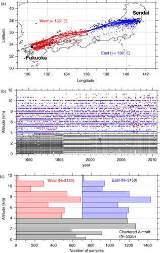
Previous studies have reported details of the Tohoku University (TU) aircraft observations for CO₂ (Tanaka et al., 1987; Nakazawa et al., 1993b), N₂O (Ishijima et al., 2001, 2010) and O₂/N₂ (Ishidoya et al., 2012). To collect air samples using aircraft, two programs have been conducted (Fig. 1). (1) For air sampling at altitudes below 4 km, a chartered aircraft (Cessna 172) was used. The aircraft took off Sendai Airport (38.13°N, 140.92°E) in the daytime under fine weather conditions and flew over the Pacific Ocean 20–50 km off the coast of the Sendai plain for about 2 hours to make a sample collection at 16 assigned altitudes. The time of air sampling was chosen mainly to ensure the safety of the flight, but such conditions allowed us to collect air representative of the large-scale atmospheric motion (high pressure conditions). At each altitude, outside air was introduced into the cabin through Tygon tubing and pressurised at ~0.3 MPa above ambient pressure into a 350 mL stainless-steel flask using an electric diaphragm pump. (2) At altitudes above 4 km, air samples were collected on board commercial jet airlines (McDonnell-Douglas MD-80 and MD-90) between Sendai and Fukuoka (33.58°N, 130.45°E), which were operated by Japan Air Systems (the former Toa Domestic Airlines) until 2004 and then by Japan Airlines. Outside air, which is introduced into the cockpit through an air-conditioning system of the aircraft, was collected at ~0.3 MPa above the cockpit pressure into a 350 mL stainless-steel flask by using a manual plunger pump developed at TU. Air sampling positions and altitudes were recorded from flight instruments of the aircraft. During a set of outbound and returning flights, 20 air samples were collected. Prior to use the flasks used in the two programs were evacuated to lower than 1.3×10⁻⁴ Pa at 120°C for at least 1 hour. Our air sampling programs are on-going with a half-year interruption after the Tohoku earthquake and tsunami in March 2011, by which Sendai Airport was seriously damaged.

Fig. 1 (a) A map showing air sampling locations by commercial aircraft (red and blue symbols) and an approximate position for sampling by chartered aircraft (black diamond). Data on board commercial aircraft are classified into west (red) and east (blue) sides. Black squares show the locations of Sendai and Fukuoka airports. (b) An altitude–time cross section for the coordinates of all available CH₄ concentration data. (c) Histograms showing number of data points at the respective altitude bins. Note that the histogram for the east data (blue) is shifted for ease of viewing.

Flasks filled with sample air were returned to our laboratory, and then analysed for CH₄ within a few days after collection using a gas chromatograph equipped with a flame ionisation detector (GC-FID). We used a GC-9A (Shimadzu Corp.) system in earlier years (Aoki et al., 1992) and replaced it with a new one (Agilent 6890, Agilent Technologies, Inc.) in 2001 (Umezawa et al., 2012a). Repetitive calibrations of the CH₄ standard gases indicated that repeatability of our measurements is 3 ppb for the GC-9A system and 2 ppb for the Agilent 6890 system. The CH₄ concentration was determined against the TU scale, which is based on primary standard gases prepared with uncertainties of 1 ppb using a gravimetrical method with four dilution stages (Aoki et al., 1992). We confirmed by regularly performing an intercalibration of our standard gases that our scale has been stable within our analytical repeatability for the period covered by the present observation programs. Results of the 5th WMO (World Meteorological Organization) Round Robin intercomparison programme (http://www.esrl.noaa.gov/gmd/ccgg/wmorr/results.php?rr=rr5&param=ch4) and additional intercomparisons conducted by JMA (Japan Meteorological Agency) (Takahashi et al., 2013) have suggested that, in the CH₄ concentration range of 1700–1900 ppb, the TU scale is ~3 ppb higher than the WMO CH₄ mole fraction scale (Dlugokencky et al., 2005).

The altitude and time coverage of CH₄ data analysed in this study are shown in Fig. 1b. The number of the CH₄ data points is also shown as histograms with respect to altitude (Fig. 1c). We classified the CH₄ data into 12 altitude levels, and the data above 4 km were further grouped into western and eastern parts of Japan. As seen in Fig. 1, regular measurements had been made over 1988–2010, providing hundreds of the CH₄ data at each altitude level. Since cruise altitudes of commercial aircraft (typically from 7 to 11 km between Sendai and Fukuoka) depend on weather conditions, air sampling altitudes were different from flight to flight. As a result, our data above 4 km are unevenly distributed on the altitude–time domain and monthly air sampling was not achieved regularly particularly at the top altitude level (Fig. 1b). On the other hand, below 4 km, air sampling using chartered flights provided data at regular altitude and time intervals. It is noted that observations differ in air sampling positions below and above 4 km. While air samples at the lower levels were collected within the relatively narrow area near Sendai, those at the higher levels were done between Sendai and Fukuoka. The air sampling locations differ up to ~4° and ~6° in latitude and longitude within the western and eastern parts of Japan, respectively, and thus represent more diverse air mass origins.

2.2. Data analyses

To extract a long-term trend, an interannual variation and a seasonal cycle from temporally discrete CH₄ concentration data, a digital filtering technique (Nakazawa et al., 1997) was applied for data at each altitude level. The technique consists of stepwise calculation process involving linear interpolation, Reinsch-type cubic splines, Fourier harmonics and a Butterworth filter. In this study, the Butterworth filter with a cutoff period of 60 months was used to derive the long-term trend, and the average seasonal cycle was expressed by fundamental and its first harmonics. Signals with periods of 4–60 months, obtained by further applying the Butterworth filter with a cutoff period of 4 months, were defined as short-term variations. The best-fit curve to the observed data was thus obtained by summing the long-term trend, average seasonal cycle and short-term variations. The data lying outside three standard deviations were excluded as outliers in the fitting procedures.

Stratosphere–troposphere exchange (STE) is one of the important factors controlling the CH₄ concentrations in the UT. The MD-80 and MD-90 aircraft frequently encounter STE events or intersect the tropopause at their cruise altitudes over Japan particularly in January–April, in association with tropopause breaks, tropopause folds and seasonal descent of the tropopause (Ishijima et al., 2010). To better represent tropospheric CH₄ variations, we excluded such STE-influenced data based on N₂O concentrations measured concurrently (details for N₂O are in Ishijima et al., 2001). The atmospheric N₂O concentration is increasing almost linearly at a fairly constant rate of 0.7 ppb yr⁻¹ over the observation period due to continued increase in anthropogenic emissions. N₂O has an atmospheric lifetime of ~120 yr (destroyed by photolysis and reaction with O(¹D) in the stratosphere) (e.g. Volk et al., 1997) and relatively well mixed in the troposphere without any measurable loss mechanism (e.g. Prinn et al., 1990; Ishijima et al., 2010). As a result, the N₂O concentration has a sharp gradient around the tropopause, allowing us to detect STE events by low N₂O concentrations (Ishijima et al., 2010; Assonov et al., 2013). Detection of STE-influenced samples was made as follows. (1) The N₂O concentration data at the respective altitude levels were detrended using the above curve fitting technique (see Fig. A1 in Supplementary file for the N₂O concentrations above 4 km). (2) Histograms of the detrended N₂O below 6.0 km could be approximated by normal distribution with width (σ) of up to 1.1 ppb (Fig. A2 in Supplementary file), which is comparable to the amplitude of the N₂O seasonal cycle in the LT over the extra-tropical regions (Prinn et al., 1990; Ishijima et al., 2001). Histograms at higher altitudes were skewed to the lower concentration side due to a significant number of STE-influenced samples. (3) The N₂O concentration data lower by more than 2.7 ppb (3σ at altitudes 4–6 km over eastern Japan) than the long-term trends were defined as STE-influenced samples (open circles in Figure A1 in Supplementary file). In general, the STE events are frequent above 7 km over Japan (Ishijima et al., 2010). It is noted that the N₂O criterion in this study is less restrictive than that of 1.0 ppb in Assonov et al. (2013), who also applied a similar method for analysing data taken by passenger aircraft. We infer that the following data analyses may be partly influenced by shallow stratospheric air at the high altitude levels. (4) Corresponding CH₄ data of the STE-influenced samples were excluded in subsequent analyses. It should also be noted that our N₂O measurement was started in 1992 and CH₄ data obtained earlier were not examined for the above STE detection. Given that the STE occurrences have clear seasonality, we discuss seasonal cycles of CH₄ based only on data screened with the N₂O measurements to minimise the STE effect to the seasonal CH₄ cycle.

2.3. Atmospheric chemistry transport model

We employed the CCSR (Center for Climate System Research)/NIES (National Institute for Environmental Studies)/FRCGC (Frontier Research Center for Global Change) Atmospheric General Circulation Model-based Chemistry Transport Model (ACTM) for simulating CH₄ concentration (Patra et al., 2009). The simulations follow the TransCom-CH₄ experimental settings (Patra et al., 2011a), but extended until 2010 with constant anthropogenic emissions after 2007. In this study, four CH₄ emission scenarios (S0, S1, S2 and S3) were prepared by combining various emission databases. Cyclostationary natural emissions (emissions vary seasonally with repeating the annual total) are prepared based on the Goddard Institute for Space Studies (GISS) inventory (Matthews and Fung, 1987; Fung et al., 1991) for the S0 and S3 scenarios, and interannually changing anthropogenic emissions are taken from the Emission Database for Global Atmospheric Research (EDGAR, version 3.2/FT) inventory (Olivier and Berdowski, 2001) for the S0, S1 and S2 scenarios. An updated EDGAR database (version 4.0) replaced the earlier version for S3. Thus the S0 and S3 simulations have interannual variations in anthropogenic fluxes but not in natural fluxes. In the S1 simulations, however, interannual variations of CH₄ flux were considered for emissions from wetlands and rice paddies based on the Vegetation Integrative Simulator for Trace gases (VISIT) terrestrial ecosystem model (Ito and Inatomi, 2012), in which a wetland emission scheme by Cao et al. (1996) was employed. Interannual variations for biomass burning emissions were taken from the Global Fire Emission Database (GFED version 3) (van der Werf et al., 2010). In the S2 simulation, the wetlands and rice emissions were simulated by VISIT, but a wetland scheme by Walter and Heimann (2000) was used. In this paper, we present simulation results with the scenarios S1, S2 and S3, which is sufficient to evaluate fundamental features seen in the present observations. It was assumed that atmospheric CH₄ is destroyed by reacting with OH, Cl and O(¹D), and the tropospheric OH field (Spivakovsky et al., 2000) was scaled so that ACTM can reproduce long-term trends of methyl chloroform (M. Krol, personal communication; as discussed in Patra et al., 2011a). The soil sink was prescribed as a climatological negative flux with seasonality (see Patra et al., 2011a). Meteorological fields in the model were nudged to Japanese 25-yr ReAnalysis (JRA25) (Onogi et al., 2007) and thus interannually variable. Patra et al. (2009, 2011a) showed that the CH₄ concentration variations observed at surface baseline stations around the world were reproduced relatively well by using this model. The model outputs were sampled for the dates, time within 1 hour and within 1.45 degree for locations (latitude/longitude) specified by our observations. Model results were vertically interpolated to the observation altitudes. Comparisons between the model and observation results for the present observation locations are presented in Fig. A3 in Supplementary file.

In addition, to examine which source regions are important at different altitude levels over Japan, tagged tracer experiments were performed using the ACTM in the same manner as mezawa et al. (2012b). The original surface flux field (S0) was divided into 15 source regions (see Fig. A4 in Supplementary file), and each CH₄ tracer was simulated separately with each flux field to explore contributions of the individual source regions to CH₄ variations at the observation locations. We confirmed that the sum of the 15 tracers and the simulated concentration with original global flux field agreed with each other within 0.1%. The tagged tracer simulation period is 2005–2010 for this analysis. The model output was sampled at observation time and locations by linear interpolation.

3. Results and discussion

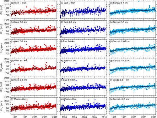
Figure 2 shows temporal variations of the CH₄ concentration at the respective altitude levels over Japan. At higher altitudes, STE-influenced air (mostly low CH₄ values) is frequently encountered in winter–spring, and extremely high CH₄ concentrations are measured commonly in summer. At the mid- to high-altitude levels (5–7 km), large variability is seen without clear seasonality, due to competing contributions from high and low CH₄ values in summer, which are respectively more pronounced at the higher and lower altitudes. As described later, the former is primarily influenced by Asian sources and the latter by enhanced chemical loss of CH₄ in summer. In the LT (Fig. 2n–s), irregular variations (seen as deviations from the best-fit curve) are smaller and clear seasonal minima in summer are obvious (see also Figs. 5 and A3 in Supplementary file). These differences in CH₄ variations with altitude are mainly due to altitude-dependent air mass origins. Namely, in the LT, the aircraft sampled air masses originating in Japan, the Japan Sea or the Pacific Ocean, while, in the mid-troposphere to the UT, high CH₄ plumes arrive over Japan from the Asian continents during the spring and summer (e.g. Xiao et al., 2004; Schuck et al., 2012).

Fig. 2 Temporal variations of CH₄ concentrations over (a)–(f) western and (g)–(m) eastern Japan observed using commercial aircraft and (n)–(s) over the Sendai area using chartered aircraft. Data influenced by STE events are identified using N₂O data measured concurrently and shown as open circles (see Fig. A1 in Supplementary file). Data obtained before initiating N₂O measurements are shown in black and are not applied for the above STE analyses. The best-fit curve (thin black line) and long-term trend (thick black line) were calculated based on data not influenced by STE events screened with N₂O data.

3.1. Long-term trend and interannual variations

Figure 3 shows long-term trends and growth rates of the CH₄ concentration at selected altitudes over Japan. Their altitude–time cross-sectional representations are also given in Fig. 4, together with those from the simulations. In the LT, the observed long-term trends were similar to previous measurements at surface baseline sites in the northern hemisphere (e.g. Dlugokencky et al., 2011). Namely, the LT CH₄ concentration over Japan showed high increase rates of more than 10 ppb yr⁻¹ in the late 1980s and the increase slowed in the early 1990s, after which the near-zero increase continued in 2000s with interannual variations, but increases of more than 5 ppb yr⁻¹ appeared again since 2007. On the other hand, the growth rates above 4 km frequently show features different from those below 4 km. This would reflect altitude-dependent air-mass origins and thus spatial representativeness of the air masses sampled change with altitude. However, it is noted that the long-term trends deduced by the curve fitting rely on the observation data that were not dense particularly at the top altitude levels (Fig. 1), which might have affected part of apparent features in the UT.

Fig. 3 Observed (black) and simulated (S1 in red, S2 in blue and S3 in green) CH₄ trend (thin solid lines) and growth rate (GR, thick solid lines) at selected altitudes over Japan.

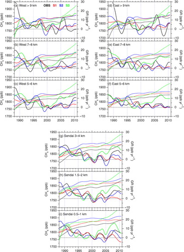
Fig. 4 Altitude–time cross sections of the long-term trend (left two columns) and growth rate (right two columns) of CH₄ over Japan obtained from observations (uppermost panels) and the three ACTM simulations (lower panels).

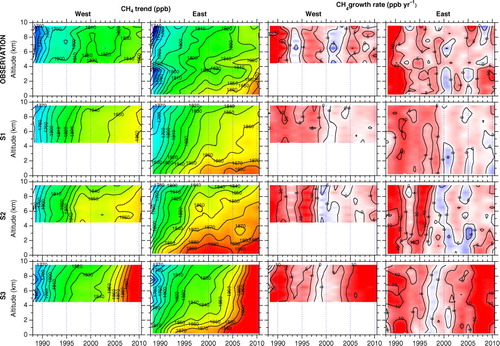
It is clearly seen in Fig. 4 that the CH₄ concentration decreases with altitude and the long-term increase over the last 20 yr at lower altitudes has preceded that at higher levels. In general, the S1 simulation best reproduces the declining growth rate in the early 1990s and the following stabilisation in 2000s. The S2 shows an overestimated increase in 1995–1996, while it matches best the growth after 2007. The S3 shows clear secular increase since mid-2000s when the observed CH₄ concentration remained almost constant (see also Fig. 3).

The growth rate of the CH₄ concentration declines during 1992–1993. This feature is more obvious over western Japan compared to the east. Such a drop in the CH₄ growth rate has been observed globally (Dlugokencky et al., 1994). Possible causes are a reduction in fossil fuel related emission in the former Soviet Union (Dlugokencky et al., 1994), a decrease in biomass burning in the tropics (Lowe et al., 1997), and a negative anomaly in emissions from northern high latitude wetlands (Walter et al., 2001). An inversion study suggested that emission reductions in wetlands as well as fossil fuel related emissions predominantly contributed to the growth rate anomaly (Bousquet et al., 2006). In this respect, the S2 simulates the declined growth rate better than S1. As described earlier, the VISIT model was used to estimate the wetland emissions for the ACTM, and different wetland schemes were employed for S1 and S2. Since the S2 wetland scheme has higher temperature sensitivity than S1, the S2 has a stronger negative anomaly in wetland emissions for 1992 (A. Ito, personal communication), and is consistent with Walter et al. (2001). This would explain the differences in ACTM's reproducibility of the growth rate for this period.

In 1995–1996, a moderate increase is observed particularly at higher altitudes over western Japan. The S2 simulation gives high growth rate (>10 ppb yr⁻¹) in the whole troposphere for the period, while the S1 results do not behave similarly. The VISIT emissions in S2 showed positive anomalies in wetland regions in North America (Hudson Bay Lowlands). It is also noted that the S3 scenario with cyclostationary natural emissions does not reproduce the observed increase during the period.

The observation shows a relatively high growth rate (5–10 ppb yr⁻¹) at most altitude levels in 1997–1998. This increase rate is smaller than that reported for the global average based on the other surface measurements (~15 ppb yr⁻¹) (Dlugokencky et al., 2001, 2011; Langenfelds et al., 2002; Simpson et al., 2002, 2006); however, ship observations in the western Pacific (Terao et al., 2011) reported moderate increase rates (5–10 ppb yr⁻¹) at mid-latitudes, being consistent with the present observation. In this connection, Patra et al. (2009) indicated that interannual CH₄ variations could be different from site to site depending on meteorological patterns. As shown in Figs. 3 and 4, the S1 simulation reproduces the high growth rate in 1997–1998 best. This emission scenario for the period consists of higher emissions from wetlands and biomass burning, compensating faster removal of CH₄ by OH due to high temperature anomaly induced by the El Niño event (Patra et al., 2011a). Previous studies also suggested that the high CH₄ growth rate is attributable to combination of positive anomalies of wetland and biomass burning CH₄ emissions (Dlugokencky et al., 2001; Bousquet et al., 2006; Morimoto et al., 2006; Hodson et al., 2011), while another study suggested that anomalous CH₄ emissions from biomass burning alone explain most of the atmospheric CH₄ increase (Simpson et al., 2006).

From 1999 to 2005, the CH₄ concentration shows almost no increase in the 2000s in the whole troposphere over Japan. The S1 and S2 simulations with no significant changes in total CH₄ emissions over the period reproduce the near-zero growth rate in the 2000s. Based on inverse modelling, Bousquet et al. (2006) suggested that low CH₄ emissions from boreal wetlands due to dry conditions competed with a coincident increase in anthropogenic CH₄ emissions in Asia, resulting in the near-zero increase in the early 2000s. Reflecting the assumed high growth of the Chinese economy, the S3 simulation with EDGAR version 4.0 inventory results in persistent increase of the CH₄ concentration after the mid-2000s. The inconsistency with the observation calls for improvement of the EDGAR4.0 (and updated EDGAR4.2, which is similar to the 4.0 version) inventory used in this scenario. This has been pointed out by Patra et al. (2011a), and recently, Bergamaschi et al. (2013) and Tohjima et al. (2014) also indicated that the emission trend in the EDGAR 4.2 inventory is likely overestimated. It is noted that our observations are under strong influence from East Asia for which anthropogenic emissions are different between the S3 and other scenarios.

In 2005–2006, high growth rates are observed in the UT over both the western and eastern part of Japan (Figs. 3 and 4). High CH₄ values observed in summer for the period resulted in the high growth rate. However, this feature is not well captured by all the simulations. We therefore cannot suggest any possible causes of the increase. We note that the observed summertime high values, which contributed to the observed high growth rates, are plausibly influenced by air masses originating in Asia as discussed later.

The observed CH₄ regrowth since 2007 is clear in the LT (~10 ppb yr⁻¹), the growth rate being similar to those reported previously by surface measurements (Rigby et al., 2008; Dlugokencky et al., 2009; Terao et al., 2011). On the other hand, the growth rate in the UT over Japan (<5 ppb yr⁻¹) is much smaller or not obvious. In this connection, Umezawa et al. (2012b) reported the growth rate of ~15 ppb yr⁻¹ in the UT over the northern western Pacific, a region south of the present observation. The difference might be attributable to larger variability over the present observation area due to more frequent encounters with high CH₄ spikes, which could have obscured changes in baseline air, and/or due to different air mass origins. The S2 simulation reproduces the 2007 increase best (Figs. 3 and 4). It is noted that the VISIT model in S2 shows positive source anomalies in South/East Asia and Northern America for 2007–2008. Previous studies attributed the 2007 increase of the atmospheric CH₄ to elevated emissions in boreal wetlands (Rigby et al., 2008; Dlugokencky et al., 2009; Sasakawa et al., 2010, 2012) as well as in tropical wetlands (Bousquet et al., 2011; Umezawa et al., 2012b; Bergamaschi et al., 2013). We note that the observed growth rate is larger than that predicted by the S2 simulation. This implies that the increase in anthropogenic emission in East Asia, as was given in the S3 simulation, could have also contributed to the renewed CH₄ growth rates since 2007.

3.2. Seasonal cycle

Figure 5 presents the observed and simulated average seasonal cycles of the CH₄ concentration below 4 km over the Sendai area. The CH₄ concentration shows clear seasonal minimum in August, as well as relatively high values in winter–spring. The phase of seasonal cycle changes insignificantly with altitude. Such seasonal minima in August have been observed at mid-latitude surface sites (e.g. Cunnold et al., 2002). Tohjima et al. (2002) reported slightly earlier CH₄ minima (late July) based on high-frequency measurements at stations Ochi-ishi and Hateruma in Japan. The differences are presumably due to different data density and air mass representativeness at the respective observation places. In general, seasonality of the CH₄ concentration is driven by seasonal change in atmospheric OH density, CH₄ emissions and atmospheric transport. At northern mid-latitudes, OH peaks in early summer (June–July), contributing to minima of the CH₄ concentration in late summer (e.g. Dlugokencky et al., 1995). Using backward trajectory information, Yashiro (2007) inspected the origin of air masses arriving at different altitude levels over the present observation area. In summer, when air in the LT originates predominantly from the Pacific Ocean or regions around Japan, oceanic air with low CH₄ concentrations combined with the enhanced OH loss in this season result in the observed CH₄ minimum. In contrast, in winter–spring, the LT air over the observation area mainly originates from the continent (northern China and Siberia). Anthropogenic CH₄ emissions under low OH loss in that season explain the observed high CH₄ levels. The importance of the air transport patterns on the trace gas variability over Japan has been discussed also in previous studies (e.g. Tohjima et al., 2002; Wada et al., 2011; Ishidoya et al., 2012; Shirai et al., 2012).

Fig. 5 Average seasonal cycles of CH₄ concentrations observed (black) and simulated (colours) below 4 km over the Sendai area.

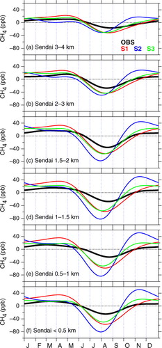
Also shown in Fig. 5 are the ACTM simulation results. The S1 simulation reproduces the timing of the observed seasonal minima best at the respective altitude level, while S2 results in about half-month earlier minima. In this regard, we note that the simulated CH₄ with the different scenarios show a seasonal minimum similar in phase, but differing in increase after the summertime minimum (Fig. A3 in Supplementary file), resulting in the apparent phase shifts deduced by the curve fitting (Fig. 5). The difference between models and observation becomes more prominent near the surface. This suggests that summertime emissions from wetlands and rice paddies in the surrounding area of Sendai, which are given differently between the scenarios, play an important role in the lowermost layers. We also note that the general overestimation of CH₄ concentration during autumn–winter by the model (Fig. A3 in Supplementary file) gave larger seasonal amplitudes in the simulations than in the observation (Fig. 5).

The present observations show that the average peak-to-peak amplitude of the seasonal cycle in the LT is ~40 ppb on average over the observation period, with the largest amplitude at 1.5–2.0 km (~50 ppb). These amplitudes are comparable to those observed at mid-latitude stations in the northern hemisphere (Dlugokencky et al., 1997; Cunnold et al., 2002), but slightly smaller than those at the two Japanese stations (Tohjima et al., 2002). Tohjima et al. (2002) indicated that, in the surface region around Japan, seasonality of air transport patterns in association with the Asian monsoon enhances the amplitude of the seasonal CH₄ cycle. We note that our measurements were based on aircraft with lower sampling frequency and that our observation area was potentially under more substantial influence from local sources. Namely, enhanced emissions from local rice paddies in summer for instance might have raised the CH₄ level when the seasonal minimum happens, resulting in smaller seasonal amplitudes. Above 2 km, the seasonal amplitude decreases with altitude, and no clear seasonality is observable at altitudes 5–7 km (see also ^{Fig. 6}Figs. 6 and A3 in Supplementary file). At these levels, both high and low CH₄ values, which are respectively distinct features at higher and lower altitude levels, appear frequently in summer and their competing contributions resulted in the ambiguous seasonal cycles deduced by the curve fitting. The change of the seasonal amplitude with altitude is also apparent in the ACTM simulations (see ^{Fig. 5}Figs. 5 and A3 in Supplementary file).

Fig. 6 Average seasonal cycles of the observed CH₄ concentration in the mid- to upper-troposphere over (a) western and (b) eastern Japan. (c)(d) Same as (a)(b), but for the tagged tracers of South Asia. (e)(f) Same as (a)(b), but for the tagged tracers of East Asia.

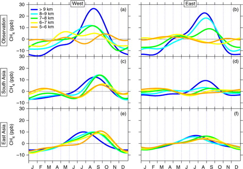
In contrast to the LT, clear seasonal maxima appear in summer at altitudes higher than 7 km. This feature is most pronounced at the highest level (>9 km) with an average peak-to-peak amplitude of ~40 ppb (Fig. 6a and 6b). The observed seasonality in the UT results from frequent appearance of high summertime CH₄ values (Figs. 2 and A3 in Supplementary file). Given that the seasonal maximum of OH density in summer is common throughout the troposphere and that the local lifetime of CH₄ is longer than a year, the observed seasonal CH₄ maxima in the UT suggest an overwhelming role of seasonal change in CH₄ emissions combined with atmospheric transport. Seasonality with summer CH₄ maxima has been also observed in the UT over the northwestern Pacific, but with double maxima in June–July and October (Matsueda and Inoue, 1996; Schuck et al., 2012; Umezawa et al., 2012b). The slightly different seasonality reflects different representativeness of air mass origins. Indeed, our tagged simulations indicate that, in early summer East Asian sources contribute less in the present observation area than in the southern area over the western Pacific.

Tagged tracer experiments are very helpful in understanding contributions from individual source regions in the altitude-dependent CH₄ seasonality over Japan. Inspecting the 15 tag regions (Fig. A4 in Supplementary file), we found that South Asia and East Asia play the largest roles in the summertime high values frequently observed in the UT. Fig. 6c–f show seasonal cycles of the tagged tracers for South Asia and East Asia at different altitude levels above 5 km. As shown in the figures, South Asia brings high CH₄ in the UT over Japan in late summer. The South Asian influence is most pronounced in the highest layers (>7 km) and larger over western Japan than in the east, while a large contribution still remains at the highest altitude in the east (Fig. 6c and 6d). The high CH₄ values originating in South Asia would be ascribed to summertime enhanced CH₄ emissions in the region (e.g. rice paddies as well as relatively constant sources such as ruminants, waste water management and biofuel burning) combined with rapid transport to the UT driven by enhanced convection over the continent. This has been also shown by previous studies using tagged tracer experiments for the northwestern Pacific (Schuck et al., 2012; Umezawa et al., 2012b) and by studies using chemistry transport models over Asian regions (Jiang et al., 2007; Park et al., 2009; Xiong et al., 2009). Air masses of boundary-layer origin in the UT over South Asia with elevated CH₄ flows out to the west due to the retreat of anticyclone over South Asia after its strongest season in July–August (Schuck et al., 2012), the air masses arriving at areas over Japan in late summer and contributing to the observed high CH₄. Previous studies also suggested that, in summer, large fraction of CH₄ emissions in South Asia originates primarily from biogenic production (Baker et al., 2012; Umezawa et al., 2012b).

As seen in Fig. 6e and 6f, tag tracers for East Asia show high contributions during early to late summer, and the influence of the region decays eastward as seen for South Asia. We note that high CH₄ values originating in East Asia appear for a relatively long period (spring to late summer), in contrast to those from South Asia, which are limited to a shorter period (late summer). In addition, it is also noteworthy that the amplitude of East Asian contribution does not vary with altitude, while South Asian influence is strongest at the highest altitude (see also Fig. 8). These features reflect the fact that East Asia is just upwind of the present observation areas. In our model scenarios, CH₄ emissions from rice paddies in East Asia peak in early summer and other important sources such as industry, ruminants and waste water management are kept constant throughout the year. These CH₄ emissions as well as enhanced vertical transport over East Asia in summer season bring high CH₄ values to the higher altitudes over Japan. The eastward decay of South Asian and East Asian outflow would be due to the transport pattern of air masses over the observation areas in associations with the prevailing westerlies.

3.3. Vertical profile

Figure 7 shows the observed and simulated vertical profiles of CH₄ concentrations over eastern Japan for different 5-yr periods (1990–1994, 1995–1999, 2000–2004 and 2005–2009). As also seen in Fig. 4, CH₄ concentrations decrease with altitude, the difference between the top and lowest altitude levels being 30–40 ppb on annual average. The vertical gradient shows no clear secular trends, although the difference between the top and lowest altitudes is slightly larger (~40 ppb) during the two periods of 1995–1999 and 2000–2004 than the other periods. The vertical profile varies with season, since the seasonal cycles are altitude dependent (Figs. 5 and 6). In winter–spring, the CH₄ decreases nearly monotonically with altitude. On the other hand, in summer–autumn, CH₄ concentrations are nearly uniform at altitudes above 2–4 km and increase with decreasing altitude in the lowermost layers. One feature seen in the vertical profiles is a dip around 2–4 km. The height with the dip in summer would be determined by balance between seasonally varying OH loss and strength of the surrounding CH₄ sources on the ground. It is also noted that there is a discontinuity in the air sampling method at 4 km (and thus rapid change of representativeness of air masses), which might have contributed to the variation in the vertical profile. In the UT, air masses with high CH₄ transported from Asian regions (Figs. 6 and 8) elevate the CH₄ concentrations in summer, resulting in the uniform vertical profile at higher altitudes. The CH₄ increase toward the surface would be due to contributions from regional/local sources (see Japan and Korea in Fig. 8).

Fig. 7 Observed vertical profiles of CH₄ concentrations over eastern Japan in different seasons during (a) 1990–1994, (b) 1995–1999, (c) 2000–2004 and (d) 2005–2009. Annual average profiles are shown in black, while colours show different seasons (red: December–February, green: March–May, light blue: June–August, blue: September–November). (e)–(h) Same as (a)–(d) but for the S1 simulation. (i)–(l) Same as (a)–(d) but for the S2 simulation. (m)–(p) Same as (a)–(d) but for the S3 simulation.

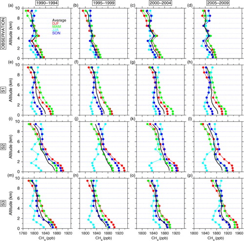
Fig. 8 (left) Observed annual-average vertical profile of CH₄ concentrations over eastern Japan (black) compared to simulated tagged tracers (colours) for different seasons for the period 2005–2009. (right) Vertical profiles of the relative contributions of the individual source regions.

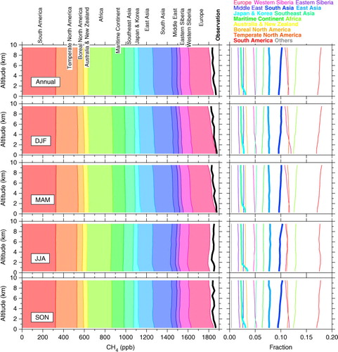
Figure 8 presents an annual-average vertical CH₄ profile obtained from the observations over eastern Japan as well as those in different seasons for 2005–2009. Those obtained from the tagged tracer simulations are also shown in the figure. Vertical profiles of relative contributions of individual tagged tracers from each source region are plotted in the right panels. General underestimation over the whole troposphere by our model is due to the emission setting that was kept constant over the simulation period, while observations showed significant increase after 2007 particularly in the LT (Figs. 3 and 4). Nevertheless, the sum of all the tagged tracers reproduces the observed vertical gradient pattern well throughout the year, allowing us to diagnose altitude-dependent contributions of individual source regions. On annual average, mid- to high-latitude source regions (Europe, Siberia and Boreal North America) have relatively higher contributions in the LT (relative contributions decrease with altitude as shown in the right panels). The relative contributions of these regions are almost proportional to the individual emission strengths due to CH₄'s long lifetime of ~10 yr, but also reflect geographical distances and air transport pattern. The adjacent region (Japan and Korea) shows a rapid increase of its relative contribution toward the surface in the lowermost layers. In contrast, relative contributions of some regions (South Asia, Africa and South America) show an increase with altitude. In summer to autumn (JJA–SON), South Asian contribution to the UT CH₄ is largest and vertical gradient of the contribution by the region becomes steeper. We also note that relative contributions of Africa and South America increase with altitude. This indicates an important role of large-scale air transport between hemispheres through the UT over the tropics (e.g. Umezawa et al., 2012b). As described earlier, the East Asian contribution shows no clear vertical gradient and seasonal dependency, showing that this upwind region has significant importance throughout the troposphere over Japan.

In general, our simulations with three different scenarios capture basic features of the seasonally dependent vertical profiles: high CH₄ values in the UT and vertical minima in the LT in summer, and nearly monotonically upward decreases in winter–spring (Fig. 7). The S1 simulation best reproduces the vertical gradient on annual average, although seasonal changes of the vertical profiles are more pronounced than the observation. In this regard, all simulations gave larger seasonal amplitudes in the LT (Figs. 5 and A3 in Supplementary file), resulting in the overestimated variation ranges in the LT. The S2 simulation shows different seasonal patterns; the vertical profile in autumn (SON) is significantly overestimated particularly in the LT, followed by the highest values in winter (DJF), resulting in the steeper vertical profiles on annual average (see also Figs. 5 and A3 in Supplementary file). As described earlier, it is very likely that CH₄ emissions from regional/local sources for the S2 scenario are overstated in summer. In the S3 simulation, the general patterns of the vertical profiles are well simulated, but significant overestimation over the whole troposphere is found in the latest time period (see also Figs. 3 and 4), reflecting the high emissions in East Asia assumed in this scenario.

4. Conclusions

We presented variations of CH₄ concentrations observed using aircraft in the troposphere over Japan during 1988–2010. The long-term trend and interannual variations in the LT are consistent with previous measurements at surface baseline sites in the northern hemisphere, while those in the UT show slightly different features from those in the LT. We also found that seasonal CH₄ cycles change with altitude over Japan. Namely, the CH₄ concentration in the UT shows a seasonal maximum in August when a seasonal minimum appears in the LT. These observed features reflect that air mass origins over Japan vary with altitude. The tagged tracer experiments indicated that the high CH₄ observed in the UT in summer is attributable to CH₄ sources in South Asia and East Asia combined with enhanced vertical transport over the continent. In addition, the ACTM simulations with three different emission scenarios reproduced the basic features of tropospheric CH₄ over Japan well, but also showed that further improvement is necessary to achieve better reproducibility of the long-term trend, seasonal cycle and vertical profile. The two simulations with different wetland emission schemes (S1 and S2) reproduced different features of the observations; S1 simulates the long-term trend and seasonal cycle better, while S2 does the interannual variations better in part. The S3 simulation using the EDGAR4.0 inventory overestimates CH₄ relative to the observations, particularly for the late 2000s, suggesting less anthropogenic CH₄ emissions in East Asia. Since the observation areas in this study are influenced by continental outflow, our CH₄ concentration data is highly valuable for improving CH₄ budget estimates in Asian regions. In particular, incorporating our data into an inversion calculation will be useful for constraining Asian emissions over the last 20 yr. The CH₄ concentration data presented in this study is available upon request for collaborative research from the principal investigators (S. Aoki and T. Nakazawa).

5. Acknowledgements

We are grateful to Japan Air System, Japan Airlines and Toho Air Service for their cooperation in collecting air samples for long years and thank all laboratory members who have been involved in the observation programs. We acknowledge A. Ito (NIES) for helpful discussions on the VISIT model. We thank A.K. Baker and two anonymous reviewers for comments to improve this manuscript.

References

- Aoki S , Nakazawa T , Murayama S , Kawaguchi S . Measurements of atmospheric methane at the Japanese Antarctic Station. Syowa. Tellus B. 1992; 44: 273–281.
- Assonov S. S , Brenninkmeijer C. A. M , Schuck T , Umezawa T . N2O as a tracer of mixing stratospheric and tropospheric air based on CARIBIC data with applications for CO2 . Atmos. Environ. 2013; 79: 769–779.
- Aydin M , Verhulst K. R , Saltzman E. S , Battle M. O , Montzka S. A , co-authors . Recent decreases in fossil-fuel emissions of ethane and methane derived from firn air. Nature. 2011; 476: 198–201.
- Baker A. K , Schuck T. J , Brenninkmeijer C. A. M , Rauthe-Schöch A , Slemr F , co-authors . Estimating the contribution of monsoon-related biogenic production to methane emissions from South Asia using CARIBIC observations. Geophys. Res. Lett. 2012; 39
- Bergamaschi P , Frankenberg C , Meirink J. F , Krol M , Villani M. G , co-authors . Inverse modeling of global and regional CH4 emissions using SCIAMACHY satellite retrievals. J. Geophys. Res. 2009; 114
- Bergamaschi P , Houweling S , Segers A , Krol M , Frankenberg C , co-authors . Atmospheric CH4 in the first decade of the 21st century: Inverse modeling analysis using SCIAMACHY satellite retrievals and NOAA surface measurements. J. Geophys. Res. 2013; 118: 7350–7369.
- Blake D. R , Rowland F. S . World-wide increase in tropospheric methane, 1978–1983. J. Atmos. Chem. 1986; 4: 43–62.
- Bloom A. A , Palmer P. I , Fraser A , Reay D. S , Frankenberg C . Large-scale controls of methanogenesis inferred from methane and gravity spaceborne data. Science. 2010; 327: 322–325.
- Bousquet P , Ciais P , Miller J. B , Dlugokencky E. J , Hauglustaine D. A , co-authors . Contribution of anthropogenic and natural sources to atmospheric methane variability. Nature. 2006; 443: 439–443.
- Bousquet P , Ringeval B , Pison I , Dlugokencky E. J , Brunke E.-G , co-authors . Source attribution of the changes in atmospheric methane for 2006–2008. Atmos. Chem. Phys. 2011; 11: 3689–3700.
- Cao M , Marshall S , Gregson K . Global carbon exchange and methane emissions from natural wetlands: application of a process-based model. J. Geophys. Res. 1996; 101(D9): 14399–14414.
- Chen Y.-H , Prinn R. G . Estimation of atmospheric methane emissions between 1996 and 2001 using a three-dimensional global chemical transport model. J. Geophys. Res. 2006; 111
- Cunnold D. M , Steele L. P , Fraser P. J , Simmonds P. G , Prinn R. G , co-authors . In situ measurements of atmospheric methane at GAGE/AGAGE sites during 1985–2000 and resulting source inferences. J. Geophys. Res. 2002; 107
- Dlugokencky E. J , Bruhwiler L , White J. W. C , Emmons L. K , Novelli P. C , co-authors . Observational constraints on recent increases in the atmospheric CH4 burden. Geophys. Res. Lett. 2009; 36
- Dlugokencky E. J , Houweling S , Bruhwiler L , Masarie K. A , Lang P. M , co-authors . Atmospheric methane levels off: temporary pause or a new steady state?. Geophys. Res. Lett. 2003; 30(19):
- Dlugokencky E. J , Masarie K. A , Lang P. M , Tans P. P , Steele L. P , co-authors . A dramatic decrease in the growth rate of atmospheric methane in the northern hemisphere during 1992. Geophys. Res. Lett. 1994; 21(1): 45–48.
- Dlugokencky E. J, Masarie K. A, Tans P. P, Conway T. J, Xiong X. Is the amplitude of the methane seasonal cycle changing?. Atmos. Environ. 1997; 31(1):21–26. Online at: http://dx.doi.org/10.1016/S1352-2310(96)00174-4.
- Dlugokencky E. J , Myers R. C , Lang P. M , Masarie K. A , Crotwell A. M , co-authors . Conversion of NOAA atmospheric dry air CH4 mole fractions to a gravimetrically prepared standard scale. J. Geophys. Res. 2005; 110: D18306.
- Dlugokencky E. J , Nisbet E. G , Fisher R , Lowry D . Global atmospheric methane: budget, changes and dangers. Phil. Trans. R. Soc. A. 2011; 369: 2058–2072.
- Dlugokencky E. J , Steele P , Lang P. M , Masarie K. A . Atmospheric methane at Mauna Loa and Barrow observatories: presentation and analysis of in situ measurements. J. Geophys. Res. 1995; 100(D11): 23103–23113.
- Dlugokencky E. J , Walter B. P , Masarie K. A , Lang P. M , Kasischke E. S . Measurements of an anomalous global methane increase during 1998. Geophys. Res. Lett. 2001; 28: 499–502.
- Etheridge D. M , Steel L. O , Francey R. J , Langenfelds R. L . Atmospheric methane between 1000 A.D. and present: evidence of anthropogenic emissions and climatic variability. J. Geophys. Res. 1998; 103: 15979–15993.
- Francey R. J , Steele L. P , Langenfelds R. L , Pak B. C . High precision long-term monitoring of radiatively active and related trace gases at surface sites and from aircraft in the Southern Hemisphere atmosphere. J. Atmos. Sci. 1999; 56: 279–285.
- Fung I , John J , Lerner J , Mattews E , Prather M , co-authors . Three-dimensional model synthesis of the global methane cycle. J. Geophys. Res. 1991; 96: 13033–13065.
- Hansen J , Sato M , Ruedy R , Lacis A , Oinas V . Global warming in the twenty-first century: an alternative scenario. Proc. Natl. Acad. Sci. 2000; 97(18): 9875–9880.
- Hodson E. L , Poulter B , Zimmermann N. E , Prigent C , Kaplan J. O . The El Niño–Southern Oscillation and wetland methane interannual variability. Geophys. Res. Lett. 2011; 38
- Houweling S , Röckmann T , Aben I , Keppler F , Krol M , co-authors . Atmospheric constraints on global emissions of methane from plants. Geophys. Res. Lett. 2006; 33: L15821.
- Ishidoya S, Aoki S, Goto D, Nakazawa T, Taguchi S, co-authors. Time and space variations of the O2/N2 ratio in the troposphere over Japan and estimation of the global CO2 budget for the period 2000–2010. Tellus B. 2012; 64 Online at: http://dx.doi.org/10.3402/tellusb.v3464i3400.18964.
- Ishijima K , Nakazawa T , Sugawara S , Aoki S , Saeki T . Concentration variations of tropospheric nitrous oxide over Japan. Geophys. Res. Lett. 2001; 28: 171–174.
- Ishijima K , Patra P. K , Takigawa M , Machida T , Matsueda H , co-authors . Stratospheric influence on the seasonal cycle of nitrous oxide in the troposphere as deduced from aircraft observations and model simulations. J. Geophys. Res. 2010; 115
- Ito A , Inatomi M . Use of a process-based model for assessing the methane budgets of global terrestrial ecosystems and evaluation of uncertainty. Biogeosciences. 2012; 9: 759–773.
- Jiang J. H , Livesey N. J , Su H , Neary L , McConnell J. C , co-authors . Connecting surface emissions, convective uplifting, and long-range transport of carbon monoxide in the upper troposphere: new observations from the Aura Microwave Limb Sounder. Geophys. Res. Lett. 2007; 34
- Khalil M. A. K , Khalil M. A. K . Atmospheric methane: an introduction. Atmospheric Methane: Its Role in the Global Environment. 2000; Berlin: Springer-Verlag. 1–8.
- Kirschke S , Bousquet P , Ciais P , Saunois M , Canadell J. G , co-authors . Three decades of global methane sources and sinks. Nat. Geosci. 2013; 6: 813–823.
- Langenfelds R. L , Francey R. J , Pak B. C , Steele L. P , Lloyd J , co-authors . Interannual growth rate variations of atmospheric CO2 and its δ 13C, H2, CH4, and CO between 1992 and 1999 linked to biomass burning. Global Biogeochem. Cy. 2002; 16
- Locatelli R , Bousquet P , Chevallier F , Fortems-Cheney A , Szopa S , co-authors . Impact of transport model errors on the global and regional methane emissions estimated by inverse modelling. Atmos. Chem. Phys. 2013; 13: 9917–9937.
- Lowe D. C , Manning M. R , Brailsford G. W , Bromley A. M . The 1991–1992 atmospheric methane anomaly: southern hemisphere 13C decrease and growth rate fluctuations. Geophys. Res. Lett. 1997; 24(8): 857–860.
- Matsueda H , Inoue H. Y . Measurements of atmospheric CO2 and CH4 using a commercial airliner from 1993 to 1994. Atmos. Environ. 1996; 30: 1647–1655.
- Matthews E , Fung I . Methane emission from natural wetlands: global distribution, area, and environmental characteristics of sources. Global Biogeochem. Cy. 1987; 1: 61–86.
- Miller J. B , Gatti L. V , d'Amelio M. T. S , Crotwell A. M , Dlugokencky E. J , co-authors . Airborne measurements indicate large methane emissions from the eastern Amazon basin. Geophys. Res. Lett. 2007; 34
- Morimoto S , Aoki S , Nakazawa T , Yamanouchi T . Temporal variations of the carbon isotopic ratio of atmospheric methane observed at Ny Ålesund, Svalbard from 1996 to 2004. Geophys. Res. Lett. 2006; 33
- Nakazawa T , Ishizawa M , Higuchi K , Trivett N. B. A . curve fitting methods applied to CO2 flask data. Environmetrics. 1997; 8: 197–218.
- Nakazawa T , Machida T , Tanaka M , Fujii Y , Aoki S , co-authors . Differences of the atmospheric CH4 concentration between the Arctic and Antarctic regions in pre-industrial/pre-agricultural era. Geophys. Res. Lett. 1993a; 20: 943–946.
- Nakazawa T , Morimoto S , Aoki S , Tanaka M . Time and space variations of the carbon isotopic ratio of tropospheric carbon dioxide over Japan. Tellus B. 1993b; 45: 258–274.
- Olivier J. G. J , Berdowski J. J. M , Berdowski J , Guicherit R , BJ Heij . Global emissions sources and sinks. The Climate System. 2001; Lisse, The Netherlands: A. A. Balkema Publishers/Swets & Zeitlinger Publishers. 33–78.
- Onogi K , Tsutsui J , Koide H , Sakamoto M , Kobayashi S , co-authors . The JRA-25 Reanalysis. J. Meteorol. Soc. Jpn. 2007; 85: 369–432.
- Park M , Randel W. J , Emmons L. K , Liversey N. J . Transport pathways of carbon monoxide in the Asian summer monsoon diagnosed from Model of Ozone and Related Tracers (MOZART). J. Geophys. Res. 2009; 114
- Patra P. K , Houweling S , Krol M , Bousquet P , Belikov D , co-authors . TransCom model simulations of CH4 and related species: linking transport, surface flux and chemical loss with CH4 variability in the troposphere and lower stratosphere. Atmos. Chem. Phys. 2011a; 11: 12813–12837.
- Patra P. K , Niwa Y , Schuck T. J , Brenninkmeijer C. A. M , Machida T , co-authors . Carbon balance of South Asia constrained by passenger aircraft CO2 measurements. Atmos. Chem. Phys. 2011b; 11: 4163–4175.
- Patra P. K , Takigawa M , Ishijima K , Choi B.-C , Cunnold D , co-authors . Growth rate, seasonal, synoptic and diurnal variations in lower atmospheric methane and its budget. J. Meteorol. Soc. Jpn. 2009; 87: 635–663.
- Prinn R , Cunnold D , Rasmussen R , Simmonds P , Alyea F , co-authors . Atmospheric emissions and trends of nitrous oxide deduced from 10 years of ALE-GAGE data. J. Geophys. Res. 1990; 95(D11): 18369–18385.
- Rasmussen R. A , Khalil M. A. K . Atmospheric methane (CH4): trends and seasonal cycles. J. Geophys. Res. 1981; 86: 9826–9832.
- Rigby M , Prinn R. G , Fraser P. J , Simmonds P. G , Langenfelds R. L , co-authors . Renewed growth of atmospheric methane. Geophys. Res. Lett. 2008; 35: L22805.
- Sasakawa M , Ito A , Machida T , Tsuda N , Niwa Y , co-authors . Annual variation of CH4 emissions from the middle taiga in West Siberian Lowland (2005–2009): a case of high CH4 flux and precipitation rate in the summer of 2007. Tellus B. 2012; 64: 17514.
- Sasakawa M , Shimoyama K , Machida T , Tsuda N , Suto H , co-authors . Continuous measurements of methane from a tower network over Siberia. Tellus B. 2010; 62(5):
- Schuck T. J , Ishijima K , Patra P. K , Baker A. K , Machida T , co-authors . Distribution of methane in the tropical upper troposphere measured by CARIBIC and CONTRAIL aircraft. J. Geophys. Res. 2012; 117
- Shirai T , Machida T , Marsueda H , Sawa Y , Niwa Y , co-authors . Relative contribution of transport/surface flux to the seasonal verztical synoptic CO2 variability in the troposphere over Narita. Tellus B. 2012; 64
- Simpson I. J , Andersen M. P. S , Meinardi S , Bruhwiler L , Blake N. J , co-authors . Long-term decline of global atmospheric ethane concentrations and implications for methane. Nature. 2012; 488: 490–494.
- Simpson I. J , Blake D. R , Rowland F. S , Chen T.-Y . Implications of the recent fluctuations in the growth rate of tropospheric methane. Geophys. Res. Lett. 2002; 29(10): 1479.
- Simpson I. J , Rowland F. S , Meinardi S , Blake D. R . Influence of biomass burning during recent fluctuations in the slow growth of global tropospheric methane. Geophys. Res. Lett. 2006; 33
- Spivakovsky C. M , Logan J. A , Montzka S. A , Balkanski Y. J , Foreman-Fowler M , co-authors . Three-dimensional climatological distribution of tropospheric OH: update and evaluation. J. Geophys. Res. 2000; 105: 8931–8980.
- Takahashi M , Nakazawa T , Aoki S , Goto D , Kato K , co-authors . Intercomparison experiments for Greenhouse Gases Observation (iceGGO) in Japan. Asia-Pacific GAW Greenhouse Gases Newsletter, Korea Meteorological Administration . 2013; 4: 45–49.
- Tanaka M , Nakazawa T , Aoki S . Time and space variations of tropospheric carbon dioxide over Japan. Tellus B. 1987; 39: 3–12.
- Terao Y , Mukai H , Nojiri Y , Machida T , Tohjima Y , co-authors . Interannual variability and trends in atmospheric methane over the western Pacific from 1994 to 2010. J. Geophys. Res. 2011; 116
- Tohjima Y , Kubo M , Minejima C , Mukai H , Tanimoto H , co-authors . Temporal changes in emissions of CH4 and CO from China estimated from CH4/CO2 and CO/CO2 correlations observed at Hateruma Island. Atmos. Chem. Phys. 2014; 14: 1663–1677.
- Tohjima Y , Machida T , Utiyama M , Katsumoto M , Fujinuma Y , co-authors . Analysis and presentation of in situ atmospheric methane measurements from Cape Ochi-ishi and Hateruma Island. J. Geophys. Res. 2002; 107
- Umezawa T , Machida T , Aoki S , Nakazawa T . Contributions of natural and anthropogenic sources to atmospheric methane variations over western Siberia estimated from its carbon and hydrogen isotopes. Global Biogeochem. Cy. 2012a; 26
- Umezawa T , Machida T , Ishijima K , Matsueda H , Sawa Y , co-authors . Carbon and hydrogen isotopic ratios of atmospheric methane in the upper troposphere over the Western Pacific. Atmos. Chem. Phys. 2012b; 12: 8095–8113.
- van der Werf G. R , Randerson J. T , Giglio L , Collatz G. J , Mu M , co-authors . Global fire emissions and the contribution of deforestation, savanna, forest, agricultural, and peat fires (1997–2009). Atmos. Chem. Phys. 2010; 10: 11707–11735.
- Volk C. M , Elkins J. W , Fahey D. W , Dutton G. S , Gilligan J. M , co-authors . Evaluation of source gas lifetimes from stratospheric observations. J. Geophys. Res. 1997; 102(D21): 25543–25564.
- Wada A , Matsueda H , Sawa Y , Tsuboi K , Okubo S . Seasonal variation of enhancement ratios of trace gases observed over 10 years in the western North Pacific. Atmos. Environ. 2011; 45: 2129–2137.
- Walter B. P , Heimann M. A . Process-based, climate-sensitive model to derive methane emissions from natural wetlands: application to five wetland sites, sensitivity to model parameters, and climate. Global Biogeochem. Cy. 2000; 14(3): 745–765.
- Walter B. P , Heimann M , Matthews E . Modeling modern methane emissions from natural wetlands 2. Interannual variations 1982–1993. J. Geophys. Res. 2001; 106(D24): 34207–34219.
- Wang J. S , Logan J. A , McElroy M. B . A 3-D model analysis of the slowdown and interannual variability in the methane growth rate from 1988 to 1997. Global Biogeochem. Cy. 2004; 18
- Warwick N. J , Bekki S , Law K. S , Nisbet E. G , Pyle J. A . The impact of meteorology on the interannual growth rate of atmospheric methane. Geophys. Res. Lett. 2002; 29
- Xiao Y , Jacob D. J , Wang J. S , Logan J. A , Palmer P. I , co-authors . Constraints on Asian and European sources of methane from CH4-C2H6-CO correlations in Asian outflow. J. Geophys. Res. 2004; 109
- Xiong X , Barnet C. D , Zhuang Q , Machida T , Sweeney C , co-authors . Mid-upper tropospheric methane in the high Northern Hemisphere: spaceborne observations by AIRS, aircraft measurements, and model simulations. J. Geophys. Res. 2010; 115
- Xiong X , Houweling S , Wei J , Maddy E , Sun F , co-authors . Methane plume over south Asia during the monsoon season: satellite observation and model simulation. Atmos. Chem. Phys. 2009; 9: 783–794.
- Yashiro H . A study of temporal and spatial variations of ropospheric carbon monoxide. 2007; Tohoku University, Sendai, Japan: Graduate School of Science. PhD thesis.