Observation of atmospheric CO₂ and CO at Shangri-La station: results from the only regional station located at southwestern China

Abstract

Mole fractions of atmospheric carbon dioxide (CO₂) and carbon monoxide (CO) have been continuously measured since September 2010 at the Shangri-La station (28.02 ° N, 99.73 ° E, 3580 masl) in China using a cavity ring-down spectrometer. The station is located in the remote southwest of China, and it is the only station in that region with background conditions for greenhouse gas observations. The vegetation canopy around the station is dominated by coniferous forests and mountain meadows and there is no large city (population >1 million) within a 360 km radius. Characteristics of the mole fractions, growth rates, influence of long-distance transport as well as the Weighted Potential CO Sources Contribution Function (WPSCF) were studied considering data from September 2010 to May 2014. The diurnal CO₂ variation in summer indicates a strong influence of regional terrestrial ecosystem with the maximum CO₂ value at 7:00 (local time) and the minimum in late afternoon. The highest peak-to-bottom amplitude in the diurnal cycles is in summer, with a value of 18.2±2.0 ppm. The annual growth rate of regional CO₂ is estimated to be 2.5±1.0 ppm yr⁻¹ (1-σ), which is close to that of the Mt. Waliguan World Meteorological Organization/Global Atmosphere Watch (WMO/GAW) global station (2.2±0.8 ppm yr⁻¹), that is also located at the Tibetan plateau but 900 km north. The CO mole fractions observed at Shangri-La are representative for both in large spatial scale (probably continental/subcontinental) and regional scale. The annual CO growth rate is estimated to be -2.6±0.2 ppb yr⁻¹ (1-σ). But the CO rate of decrease in continental/subcontinental scale is apparently larger than the regional scale. From the back trajectory study, it could be seen that the atmospheric CO mole fractions at Shangri-La are subjected to transport from the Northern Africa and Southwestern Asia sectors except for summer and part of autumn. The WPSCF analysis indicates that the western and southwestern areas of the Shangri-La station (India, Myanmar and Bangladesh) may be the most important CO sources.

• carbon dioxide
• carbon monoxide
• variations
• observation
• back trajectory

1. Introduction

Carbon dioxide (CO₂) is the most important greenhouse gas of anthropogenic origin that contributes to more than 60 % of total radiative forcing (RF) of the long-lived greenhouse gases (IPCC, 2013; AGGI, 2014). The large increase of atmospheric CO₂ of nearly 120 ppm above preindustrial levels has been unequivocally attributed to human emissions (Keeling, 1993; IPCC, 2013; WMO, 2014). This increase is mainly from fossil fuel burning and land-use changes (Houghton, 2003; Peters et al., 2012). Oceans and terrestrial ecosystems act as sinks for atmospheric CO₂ and absorb approximately half of the anthropogenic emissions (Ballantyne et al., 2012). Carbon monoxide (CO) is not a greenhouse gas as it hardly absorbs any infrared radiation from the earth. However, the reaction with hydroxyl radicals (OH) in the atmosphere, as the main sink of CO, will enhance the lifetime of other components such as methane, halocarbons and tropospheric ozone (Crutzen, 1973; Thompson, 1992; Mickley et al., 1999). As a result, it is generally considered as an important indirect greenhouse gas (Daniel and Solomon, 1998). Sources of atmospheric CO include fossil fuel combustion and biomass burning (Duncan et al., 2007) and the oxidisation of methane and other hydrocarbons (Holloway et al., 2000). Major sinks of atmospheric CO include reaction with OH and surface deposition (Seinfeld and Pandis, 1998).

China has become the number one state concerning fossil fuel CO₂ emissions in 2006 and emitted 1.8 PgC in 2011 (Marland 2012; LeQuéré et al., 2013). Along with the development of the economy, increased combustion of fossil fuels, relatively low combustion efficiency and weak emission control measures have also led to drastic increases in air pollutants such as CO and other components (Ohara et al., 2007; Lin et al., 2014).

Many background CO₂ and CO observations are made around the world under the framework of the World Meteorological Organization/Global Atmosphere Watch (WMO/GAW) programme to understand the carbon cycle in atmosphere (Keeling et al., 1976; Tans et al., 1990; Novelli et al., 2003; Artuso et al., 2009; Zhang et al., 2011; Andreae et al., 2012). In the past years, a lot of measurement campaigns or research programmes were also carried out in China (Wang et al., 2002; Gao et al., 2005; Zhou et al., 2006; Fu et al., 2009; Liu et al., 2009; Zhang et al, 2011). Most of them focussed on emissions from or concentrations in severely polluted areas. The China Meteorological Administration (CMA) is responsible for background greenhouse gas measurements. Currently, CMA is running seven stations with one WMO/GAW global station (Mt. Waliguan in Qinghai province), three WMO/GAW regional stations (Shangdianzi in Beijing, Lin'an in Zhejiang and Longfengshan in Heilongjiang province) (Fig. 1) and three Chinese regional stations (Shangri-La in Yunnan, Jinsha in Hubei and Akedala in Xinjiang province). The four WMO/GAW stations have in place in situ greenhouse gas measurement systems (for CO₂, CH₄, etc.) already for years and their observations have been thoroughly investigated along with associated data analysis, interpretation and publications (Zhou et al., 2004, 2006; Yao et al., 2012; Fang et al., 2013; Zhang et al., 2013; Fang et al., 2014; Liu et al., 2014).

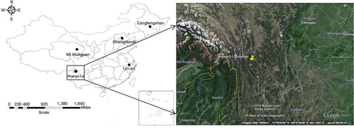
Fig. 1 Location of the Shangri-La station and the four World Meteorological Organization/Global Atmosphere Watch (WMO/GAW) stations (Mt. Waliguan global station, Shangdianzi, Lin'an and Longfengshan regional station). Currently, these stations are running with in situ CO₂/CH₄ observation systems.

To expand the observations of greenhouse gas on the Chinese mainland, a cavity ring-down spectroscopy (CRDS) analyser (G1302, Picaro Inc.) was installed in 2010 at the Shangri-La station. Since then, first-hand observations of CO₂ and CO mole fractions over the southwest of China have been acquired. In this study, we present and analyse the CO₂ and CO time series from September 2010 to May 2014.

2. Experiment

2.1. Sampling site

The Shangri-La station (28.01 ° N, 99.73 ° E, 3580 masl) is located in the Tibetan autonomous prefecture of Diqing in Yunnan province, China. The of the station is illustrated in Fig. 1. The station is ~30 km to the north of the Shangri-La town (a tourist town, ~60,000 inhabitants), which is in the joint of Yunnan, Sichuan province and Tibetan autonomous prefecture. The climate type here is tropical monsoon (Am). There are no strong anthropogenic CO₂ and CO sources such as villages, agricultural fields or factories within a 5 km radius of the station. The terrain surrounding the station is dominated by coniferous forests and mountain meadows. The population density within this area is about 10 per square kilometre, implying a weak anthropogenic influence on regional atmospheric CO₂ and CO mole fractions. The observatory is built on the top of a hill (~200 magl). A small village road runs from southwest to northeast, ~0.4 km away from the station. The road is generally for agricultural vehicles with a very light load (~10 passes per day). A sampling tower is erected next to the observatory with a height of 55 magl and the sample inlet is fixed at 50 m height. Near the sampling port, meteorological sensors (Changchun Met. Inc., Changchun, China) for wind speed, direction, atmospheric pressure, air temperature and humidity are also installed.

2.2. Measurement system

A cavity ring-down spectrometer (G1302, Picarro, Inc., Santa Clara, CA, USA) is used for continuous measurements of atmospheric CO₂ and CO. This instrument and the measurement technique have been proven to be suitable for measurements of atmospheric CO₂ and CO mole fractions (Crosson, 2008; Zellweger et al., 2012; Welp et al., 2013). The factory reported precision is 50 ppb for CO₂ and 2 ppb for CO (1-σ) in 5 min. The measurement technique is identical to and the measurement system is similar to the CRDS instruments (G1301, Picarro) for simultaneous CO₂ and CH₄ observations installed at the four WMO/GAW stations in China. Only the selected wavelengths are different adapted to the spectral properties of CO₂ and CO. The detailed schematic of measurement setup is described in Fang et al. (2013). Air sample is delivered to the instrument by a vacuum pump (N022, KNF Neuberger, Germany) via a dedicated 10-mm o.d. sampling line (Synflex 1300 tubing, Eaton, Cleveland, OH, USA). Then the ambient air is filtered (7 µm) and pressurised at 1 atm. The ambient air is dried to a dew point of approximately −60 °C by passing it through a glass trap submerged into a −70 °C ethanol bath (MC480D1, SP Industries, Warminster, PA, USA). An automated sampling module equipped with a VICI 8-port multi-position valve is designed to sample from separate gas streams (standard gas cylinders and ambient air). The effective travel time of the air from the top of inlet to the analyser is less than 45 s. The system became operational on 18 September 2010.

2.3. Calibration, quality control and data processing

The CO₂ and CO dry air mole fractions are referenced to a working high (WH) and a working low (WL) standard. Additionally, a calibrated cylinder is used as a target (T) gas to check the performance (precision and accuracy) of the system routinely. All standard gases are pressurised in 29.5 L treated aluminium alloy cylinders (Scott-Marrin Inc., Riverside, CA, USA) fitted with high-purity, two-stage gas regulators (CGA-590, Scott Specialty Gases Inc., Plumsteadville, PA, USA). The scale for CO₂ is the WMO X2007 scale (Zhao et al., 1997; Zhao and Tans, 2006) and for CO, it is the National Oceanic and Atmospheric Administration (NOAA)/WMO 2004 scale (Novelli et al., 1991). The two standards and target gas are analysed for 5 min every 6 h.

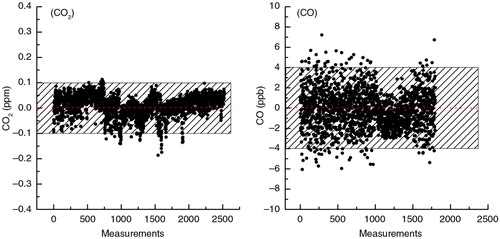
Due to the time required for flushing the internal volume of the analyser, the response of the analyser is usually not stable until 1 min after switching to a different gas stream using the multi-position valve. Every gas cylinder (WH, WL or T) is measured for 5 min. Thus, we used the last 4 min of each 5-min segment to compute CO₂ and CO mole fractions and the averages in the 4 min are used to represent the levels in current 5-min segment. The mole fractions of both gases were calibrated using a linear two-point fit through the most recent standard gas measurements (WH & WL). Figure 2 illustrates the differences between the measured and the assigned values in T. The average differences are 0.01±0.04 ppm for CO₂ and −0.2±1.9 ppb for CO during the observation period, proving that the accuracies of measurement meet the compatibility goals of WMO/GAW (0.1 ppm for CO₂ in the Northern Hemisphere and 2 ppb for CO). The 5-min data selected in that manner were then aggregated to hourly averages. To evaluate the seasonal cycle and peak-to-bottom amplitude, we used the curve fitting method described by Thoning et al. (1989) to fit the CO₂ data. In this study, the data were fitted into a function with three polynomial terms for the long-term trend and four annual harmonic terms. Except for special notes, the average values in this study are reported with 95 % confidence intervals (CI). The CO₂ and CO mole fractions in this study are in dry air.

Fig. 2 Differences of the measured and assigned CO₂ and CO mole fractions in reference tank (T) during the observation period at Shangri-La station.

3. Results and discussions

3.1. Diurnal CO2 and CO variations

Figure 3 shows the diurnal variations of CO₂ (a) and CO (b) for each of the four seasons. The corresponding months are March–May (MAM) for spring, June–August (JJA) for summer, September–November (SON) for autumn and December–February (DJF) for winter. Only days containing 24 1-h average values are considered to reduce the effect of day-to-day CO₂ and CO mole fractions fluctuations. In summer, a distinct CO₂ variation is observed with, on average, the minimum value at 17:00 (local time) and the maximum at 7:00 in the morning. The occurrence times of the minimum and the maximum CO₂ lag ~1 h behind those at Lin'an station, which is located in the east of China (Fang et al., 2014). This offset corresponds to the difference in local solar time due to Lin'an's location further east (119.44 ° E versus 99.73 ° E at Shangri-La). Thus the diurnal cycles are comparable, despite the different altitude and vegetation. Distinct CO₂ variation is also observed in autumn, reflecting that the local sources and sinks still have a large influence on observed CO₂ mole fractions (Kerang et al., 2004). The average peak-to-bottom amplitudes of the diurnal cycles are 3.4±0.8 ppm in spring, 18.2±2.0 ppm in summer, 10.2±1.2 ppm in autumn and 1.5±1.0 ppm in winter. The small diurnal variation in winter is due to the extreme low temperature (average −10 °C).

Fig. 3 Mean diurnal variations of CO₂ and CO mole fractions in the four seasons. Spring: March–May (MAM); summer: June–August (JJA); autumn: September–November (SON); winter: December–February (DJF). (a) CO₂, (b) CO versus surface wind speed. Error bars indicate the standard errors with 95 % confidence intervals.

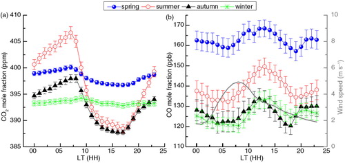
Diurnal CO variations at Shangri-La have similar patterns in all seasons, with peak values during daytime and relatively lower values during the rest of the day. The CO mole fraction reaches its maximum at 12:00–14:00. We investigated the atmospheric CO at Mt. Waliguan station (altitude 3810 masl) located on the Tibetan plateau (Shangri-La is situated at the southeastern edge and Mt. Waliguan is at the northeastern edge) during the same period and from 2004 to 2007, and the diurnal patterns in all seasons also display the maximum at 10:00–15:00, except in summer, when another peak was seen at 20:00 (Zhang et al., 2011). The enhanced values at Mt. Waliguan station are caused by upslope winds from the surrounding areas transporting pollution to the station, as also observed at mountain station Jungfraujoch in the Swiss Alps (Zellweger et al., 2009). However, the Shangri-La station is located on a plateau and the observatory is built on a relatively small hill. The higher CO values in the midday are more likely due to larger scale advection. We studied the CO mole fractions versus wind speeds during the observation period and found that the CO mole fractions were lower than 132±2 ppb when the surface wind speed was lower than 1.5 m s⁻¹ (Beaufort scale 0 & 1), and increased to 141±1 ppb above Beaufort scale 2 (> 1.6 m s⁻¹). Higher levels of CO might be transported along with these stronger winds from southwest of the observatory (see section 3.4). Most of the moments of stronger wind speed are observed in the morning with peak speed at 8:00, 4–6 h prior to the maximum CO values (grey line in Fig. 3b). The time difference between the peak in wind speed and CO concentrations is probably due to the transport time from remote CO sources.

3.2. Data filtering approaches for CO₂ and CO

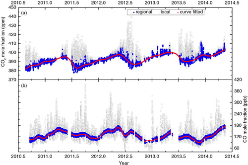
Figure 4 shows the hourly averages of the atmospheric CO₂ and CO mole fraction at Shangri-La station. The data gaps are mainly due to malfunctioning of the instrument, maintenance of the gas sampling system and unexpected power failure. (The station is located at the remote southwestern China and a robust power supply is lacking. The stationary UPS system can only last a very short period). To identify the CO₂ and CO data at least influenced by local processes adjacent to the station (by local vegetation, vehicles on road, cattle), we used methods similar to previous studies to filter the observed data into ‘regional’ and ‘local’ values (Zhou et al, 2004; Fang et al, 2013; Liu et al., 2014). Unlike the other WMO/GAW regional stations in China, the Shangri-La station is located in a remote area without obvious local anthropogenic emissions. Thus we used mainly two steps to flag the CO₂ data. First, night-time data were dismissed from the regional events to exclude episodes with significant local biospheric CO₂ respiration under poorly mixed atmospheric conditions. Second, we flagged the data when the surface wind speed was lower than 1.5 m s⁻¹ to minimise the influence of very local sources/sinks. The remainder of the data were flagged as ‘regional’ mole fractions (Fig. 4a). After the two steps filter, 8126 hourly CO₂ mole fractions are identified as ‘regional’ events, which account for ~35 % of the total valid hourly mole fractions. For CO, we applied the robust extraction of baseline signal (REBS) method to extract the regional values, which is widely used in the Global Atmospherics Gases Experiment/Advanced Global Atmospherics Gases Experiment (GAGE/AGAGE) network and other sites (e.g. Zhang et al., 2011; Ruckstuhl et al., 2012). It is a purely non-parametric technique that is used to track any long-term trend and seasonal variation. It assumes that the background signal varies very slowly relative to the contributions of the regional signal. After the filtering, about 12,780 hourly CO is identified as regional events, accounting for ~53 % of the total values (Fig. 4b).

Fig. 4 Variations of hourly CO₂ and CO mole fractions at Shangri-La station. (a) Long-term CO₂ variations. (b) Long-term CO variations. The blue closed circles are regional records and the grey open circles are local representative. The red dots in the upper chart are the curve-fitted results to the background CO₂ using the method by Thoning et al. (1989). The red dots in the lower chart are curve-fitted results to the regional CO using the Robust Extraction of Baseline Signal technique according to Ruckstuhl et al. (2012).

Table 1 illustrates the annual mean regional CO₂ and CO mole fractions at Shangri-La station and at Mt. Waliguan station in China. The CO₂ mole fractions at Shangri-La are lower than those at the other regional stations in China and are similar to those at Mt. Waliguan. The CO mole fractions at Mt. Waliguan and Shangri-La are obviously lower than those in the east of China, for example, 393±223 at Mountain Tai (Gao et al., 2005). Relatively, the CO values at Shangri-La are also lower than those of the Mt. Waliguan in the last 3 yr, especially in 2012, with a difference of ~22 ppb. It is known that atmospheric CO at Mt. Waliguan is partly influenced by transport from the heavily populated regions located at the east or southeast of the station (Tang et al., 1999; Zhang et al., 2011). While for Shangri-La station, the nearest big city is Myitkyina in Myanmar, located 360 km away, with a population of ~200,000 and Kunming in China, located 460 km away, with a population of 7 million. The lack of strong emissions from big cities near the station may be the main reason for the lower CO mole fractions.

Table 1. Annual mean regional CO₂ and CO mole fractions at Shangri-La station from 2011 to 2013, compared with the background data at Mt. Waliguan station in China

	CO2/ppm		CO/ppb
Year	Shangri-La	Mt. Waliguan	Shangri-La	Mt. Waliguan
2011	389.8±0.1	389.1±0.3	131±1	136±2
2012	393.3±0.1	392.1±0.3	139±1	161±5
2013	396.7±0.2	393.9±0.3	109±1	125±2

3.3. Seasonal variations

The red dots in Fig. 4 denote the curve-fitted results of regional CO₂ (Fig. 4a) and CO (Fig. 4b). Using the method of Thoning et al. (1989), the annual CO₂ growth rate is estimated to be 2.5±1.0 ppm yr⁻¹ (1-σ) during the observation period, which is close to that of the Mt. Waliguan station (Fang et al., 2014), and the global average during the same period as well (WMO, 2014). For CO, the yearly growth rate is −2.6±0.2 ppb yr⁻¹ (1-σ).The negative trend reflects the descending CO mole fractions over southwestern China (Tohjima et al., 2014).

Figure 5 illustrates the seasonal cycle of regional CO₂ and CO mole fractions. For comparison, the data during the same period from Mt. Waliguan are presented, as well as the surface CO₂ mole fractions from the Marine Boundary Layer (MBL) reference computed by NOAA/GMD as a function of latitude (30 deg. N). The seasonal CO₂ variation at Shangri-La is similar to that of the MBL reference, with the maximum value in May and the minimum value in August to September (Fig. 5a). The peak-to-bottom amplitude of the monthly average is 10.5±5.9 ppm, which is higher than the value of Mt. Waliguan (8.5±4.5 ppm) and the MBL (5.7±4.8 ppm). The larger amplitude at Shangri-La indicates the influence of the regional terrestrial ecosystem. The CO₂ mole fractions in spring nicely match the MBL values, while in summer, the difference of CO₂ values between Shangri-La and MBL is large with a maximum difference of 4.8 ppm in August. The almost always lower CO₂ mole fractions than MBL proves that this area averaged over the whole year acts as a regional sink of atmospheric CO₂.

Fig. 5 Monthly regional CO₂ and CO mole fractions at Shangri-La station. (a) Also compared with the monthly values at Mt. Waliguan station and surface values computed at the Marine Boundary Layer (MBL). (b) Also compared with the values at Mt. Waliguan station.

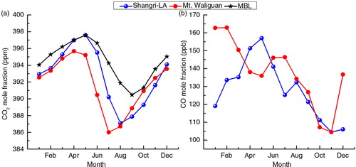
CO mole fractions at Shangri-La station display strong monthly variations. The maximum value is in May (157±1 ppb) and the minimum value (104±1 ppb) is in November. In the northern hemisphere, seasonal CO cycle is mainly driven by variations in OH abundance as a CO sink with the highest monthly value generally observed in March and the lowest value in July (Wang et al., 2010; Tohijima et al., 2014). This pattern – in particular the minimum in summer – cannot be observed at Shangri-La. It is well known that biomass burning and the combustion of fossil fuels in Southwest Asia is a very important contributor to atmospheric CO and CO₂ in the region, especially in spring (Liu et al., 2003; Streets et al., 2003; Turnbull et al., 2011; Yen et al., 2013; Jena et al., 2015). The Shangri-La station is located at the southwestern border of Chinese mainland and is isolated from the east by Hengduan Mountains and from the north by Tanggula & Himalayas Mountains in China. As most of the air masses arriving at the station are from west or southwest (e.g. India, Bangladesh and Myanmar; see section 3.4), the strong CO emissions from Southern or Southwestern Asia can be easily transported towards the station and hence induce high CO mole fractions in May. For example, most of the CO emissions from biomass burning in India are located in east–northeast and the Western Indo-Gangetic plain (Venkataraman et al., 2006), that is located at about 1800 km southwest of Shangri-La station. CO enhancement during summer has also been observed in the upper troposphere over South Asia from the CARIBIC aircraft measurements at flight (Schuck et al., 2010; Rauthe-Schöch et al., 2015). Lin et al. (2015) observed the atmospheric CO from 2007 to 2011 at the Hanle station (32.78 ° N, 78.96 ° E, 4517 masl) in India, which is located at 2000 km west of Shangri-La. They found that the CO mole fractions reached their maximum in mid-March and the minimum by the end of October and they concluded that the delay in timing of the seasonal CO minimum was due to the mixing time of regional surface CO emissions and the relatively short atmospheric lifetime of CO (1–2 months on average). On the other hand, the summer season is monsoon at Shangri-La with monthly precipitation larger than 300 mm, which will obviously reduce the oxidation capacity (O₃, OH radicals) in the regional atmosphere (Ma, 2011), leading to a subsequent lower CO sink. As a result, the mole fractions will not reach the lowest values until November. This result also confirms that, besides the influence of OH radicals, the variation of CO at Shangri-La is driven by long-distant transport.

3.4. Influence of long-distance transport on ambient CO

Back trajectories combined with long-term air measurements can be used for estimation of large scale transport and source identification (Rousseau et al., 2004). To study the contribution of regional sources on observed CO₂ and CO mole fractions, we computed 5-day back trajectories coincident with the hourly observations using the Hybrid Single-Particle Lagrangian Integrated Trajectory (HYSPLIT) dispersion model (Draxler and Rolph, 2003). The model is based on NCEP/NCAR reanalysis data. Trajectories were calculated seasonally for hours when both CO₂ and CO mole fractions were regional representative. The arrival height of the trajectories is set to 50 magl, as this is estimated to be the representative average height of the mixed layer (on the times corresponding with the selected data points).

The cluster analysis results are shown in Fig. 6. In winter and spring virtually all trajectories are from west of the station, also 44.8 % of trajectories in autumn are from these directions. These phenomena indicate that the regional CO mole fractions at Shangri-La are subjected to transport from this direction. The CO mole fractions differ on clusters and in separate seasons. For example, in winter, cluster 2 moves very fast and runs through the Southern Europe (Mediterranean Sea area), northern Africa and northern India. It has a higher mean CO mole fraction (122±1 ppb) than cluster 1 (Table 2). Cluster 1 moves over Southern Asia and northern Arabian Sea. Although both clusters run over northern India, northern India is not expected to be a major contributor to the CO levels at Shangri-La as the winter monsoon usually moves the emissions to the Indian Ocean at lower latitudes (Rauthe-Schöch et al., 2015). Cluster 2 may bring pollution from Europe to the station and induce higher mean CO mole fractions; in spring, the difference of CO mole fractions is not obvious. As the CO emissions from biomass burning are very strong in spring in Indo-Gangetic plain in India (Venkataraman et al., 2006) and both clusters run through this region, the regional CO mole fractions at Shangri-La may be primarily influenced by the emissions from this area, which subsequently leads to the highest monthly value in May (Fig. 5).

Fig. 6 Cluster analysis of 120-h back trajectories for hours when both CO₂ and CO mole fractions are regional representative. The average CO₂ and CO mole fractions on each cluster are also calculated and the relative occurrences are given. The ranges represent the standard errors of the mean with a confidence interval of 95 %. The red dots in the figure represent cities (>100,000 inhabitants).

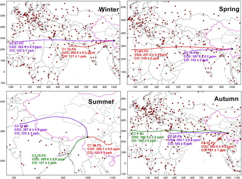
Table 2. Cluster analysis of the trajectories in all seasons and the average regional CO₂ and CO mole fractions on each cluster

Season	Cluster	Number of trajectories	Average CO2 mole fraction (ppm)	Average CO mole fraction (ppb)	Region of air mass origin	*Scale
Winter	1	601	392.8±0.3	117±1	Southern Asia, Northern Arabian Sea	CON
	2	1256	392.9±0.2	122±1	Southern Europe, Northern Africa, Southern Asia	CON
Spring	1	187	397.0±0.4	140±2	Southern Europe, Northern Africa, Southern Asia	CON
	2	547	397.5±0.2	142±2	Southern Asia	CON
Summer	1	81	388.1±0.9	133±3	Developed area in China (Guangxi and Guizhou province in China)	REG
	2	99	387.8±0.9	125±2	Tibetan plateau	REG
	3	97	389.6±0.6	127±2	Southern Asia	REG
Autumn	1	296	386.9±0.3	121±1	Bangladesh, Myanmar, northeastern India	CON
	2	191	390.1±0.6	105±2	Southern Asia, border of Tibetan plateau	REG
	3	49	390.5±1.0	100±5	Southern Europe, Northern Africa, Southern Asia	REG

*CON represents mole fractions may be influenced by air masses from continental/subcontinental scale, and REG represents values mainly influenced by air masses from REGIONAL scale.

In summer and autumn, the CO mole fractions are more influenced by regional sources compared with the other seasons. Cluster 1 (29.2 %) runs from some of the developed areas in China (Guangxi and Guizhou province). It has the highest CO mole fraction (133±3 ppb). Cluster 2 crosses the Tibetan plateau, which is commonly considered as a ‘clean’ and isolated area (Zhou et al., 2006). The average CO mole fractions are obviously lower than the others. Most of the trajectories in autumn are from the southwest of the Shangri-La (55.2 %). Cluster 1 is from Bangladesh, Myanmar, and the northeastern India where several big cities are located (Chittagong and Khulna in Bangladesh, Kolkata in India). Average CO mole fraction on it is the highest with a value of 121±1 ppb.

3.5. Scale representative of the filtered mole fractions

In general, the CO mole fractions at Shangri-La are influenced by air masses from two scales. One is at the continental/subcontinental scale (CON), from east of the station, including Southern Europe, Northern Africa and Southern Asia, which is mostly observed in winter, spring, and partly in autumn. The other is at the regional scale (REG), from southeast (developed region), northwest (poorly developed area) and southwest of the station (Bangladesh, Myanmar and the northeastern India). Thus the CO mole fractions in winter, spring and cluster 2 & 3 in autumn are defined as CON events, and the rest of them are REG events. The CO growth rates calculated from the liner regressions are −9±1 ppb yr⁻¹ at CON scale and −2±1 ppb yr⁻¹ at REG scale. The smaller CO decreasing rate in REG indicates that Southeast Asia may still act as a source of atmospheric CO (Jena et al., 2015).

Unlike to the CO, the differences of average CO₂ mole fractions among the clusters in all seasons are not evident, except for the extremely slow moving cluster 1 in summer. Besides the long-distance transport, atmospheric CO₂ mole fractions are affected by many factors such as regional anthropogenic sources, absorption/emission by regional terrestrial ecosystems, short/medium range transport, etc. The CO₂ records at Shangri-La can be used in inverse or transport models (e.g. Carbon-Tracker) to evaluate regional sources/sink strength within the Southwest China, Bangladesh, Myanmar and northeastern India region. While for CO, the records may be assimilated in models to evaluate sources/sink in continental/subcontinental and regional scale respectively, as it is influenced by a very large region.

3.6. Potential sources contribution of CO

To identify the potential source area of CO, we used the potential sources contribution function (PSCF) analysis which was previously used at the Mt. Waliguan station (Zhang et al., 2011). This method can calculate the probability density functions reflecting the residence times of an air parcel over a given geographical area prior to its arrival at the observatory using back trajectories (Begum et al., 2005). Details of this method are described in Li et al. (2012). When calculating PSCF values, some grid cells will contain only 1 endpoint (n _ij =1). If this endpoint happens to be a ‘pollution’ event, the PSCF will be 1. Thus there is a bias on the estimation. To reduce this large uncertainty, a weighted function W(n _ij ) was multiplied by the PSCF as used in previous studies (Polissar et al. 1999; Wang et al., 2009) (WPSCF). Here, W(n _ij ) was defined as:

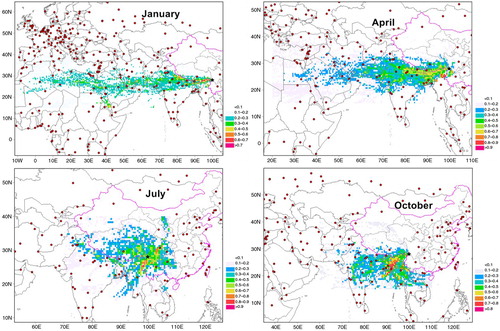
The geographical region covered by the trajectories is divided into 0.5×0.5 degree grid cells (with a height of up to 500 magl). The data in January, April, July and October are used to calculate WPSCF. The average regional CO mole fractions in the selected respective month were used as the thresholds to defined ‘pollution’ events. Figure 7 shows the potential sources region from back trajectory statistics. In winter, the sources contributing to the CO mole fractions are likely to be located within a continental/subcontinental region (from Southern Europe, Northern Africa to Southern Asia), and most CO sources are located in northern Myanmar and Nepal. In spring, besides the potential regions concluded in section 3.4, there is a possible contribution from the city of Myitkyina in Myanmar located at southwest of the station. On the other hand, the high CO emissions from the biomass burning and fossil fuel combustion in this area may induce the highest CO mole fraction in May at Shangri-La. The potential sources in summer are more restricted within the regional areas than in the other seasons with two main directions. One is from the southwest (Myitkyina in Myanmar, and Lijiang in Yunnan province, China), and the other is from the northeast of the station, where the megacities of Chengdu (516 km away) and Chongqing (690 km away) in China are located. In autumn, the high CO mole fractions are likely from southwest of the station (Myanmar, Bangladesh and northern India). Overall, except in summer, the CO mole fractions observed at Shangri-La station are mainly subject to transport from the west or southwest of the station, from Southern Europe, Northern Africa to Southern Asia. It should be noted that the WPSCF method only studies the possibility of CO sources and there may also be errors for the simulation because it only considers back trajectories. For example, there is potentiality of CO from the Bay of Bengal in the four seasons, especially for the simulation in October. Obviously, the ocean cannot be a strong source of atmospheric CO.

Fig. 7 The Weighted Potential CO Sources Contribution Function (WPSCF) regions calculated from trajectory statistics in January, April, July and October during the observation period (from September 2010 to May 2014). The WPSCF values have an arbitrary unit; higher value indicates a higher probability for a grid cell of CO sources (the largest value is 1). The red dots on the map represent big cities.

4. Conclusions

Atmospheric CO₂ and CO mole fractions measured at Shangri-La station located in southwestern China have been reported. Characteristics of the mole fractions, growth rates and the influence of long-distance transport, as well as the WPSCF, were studied. Atmospheric CO₂ mole fractions at Shangri-La are affected by regional terrestrial ecosystems. The annual CO₂ growth rate and the seasonal variation at Shangri-La are similar to those of the Mt. Waliguan WMO/GAW global station. The CO mole fractions observed at Shangri-La represent a larger scale (probably continental/subcontinental) than CO₂ because this site is relatively remote and there are no strong anthropogenic emissions within a 360 km radius. From the trajectories study, it could be seen that the atmospheric CO at this station is mainly subject to transport from Northern Africa, Southern Europe and Southern Asia except for summer. The WPSCF analysis shows that the western and southwestern area of the Shangri-La (India, Myanmar, Bangladesh) may be the most potential CO sources. In this study, we only present 4 yr of continuous atmospheric CO₂ and CO measurements at Shangri-La station. Future analysis which can profit from the ongoing observations and thus, longer time series will help to better understand the underlying processes.

5. Acknowledgements

We express our thanks to the staff at Shangri-La station, who have contributed to the system installation and maintenance. This work is supported by National Natural Science Foundation of China (No. 41375130, 41405129, 41303052). Martin Steinbacher acknowledges funding from QA/SAC Switzerland which is financially supported by MeteoSwiss and Empa.

References

- AGGI. NOAA Earth System Research Laboratory, Boulder, CO. The NOAA Annual Greenhouse Gas Index (AGGI). 2014. Online at: http://esrl.noaa.gov/gmd/aggi/.
- Andreae M. O. , Artaxo P. , Beck V. , Bela M. , Freitas S. , co-authors . Carbon monoxide and related trace gases and aerosols over the Amazon Basin during the wet and dry seasons. Atmos. Chem. Phys. 2012; 12: 6041–6065.
- Artuso F. , Chamard P. , Piacentino S. , Sferlazzo D. M. , Silvestri L. D , co-authors . Influence of transport and trends in atmospheric CO2 at Lampedusa. Atmos. Environ. 2009; 43: 3044–3051.
- Ballantyne A. P., Alden C. B., Miller J. B., Tans P. P., White J. W. C. Increase in observed net carbon dioxide uptake by land and oceans during the past 50 years. Nature. 2012; 488: 70–73.
- Begum B. A. , Kim E. , Jeong C. H. , Lee D. W. , Hopke P. K . Evaluation of the potential source contribution function using the 2002 Quebec forest fire episode. Atmos. Environ. 2005; 39: 3719–3724.
- Crosson E. R . A cavity ring-down analyzer for measuring atmospheric levels of methane, carbon dioxide, and water vapor. Appl. Phys. B. 2008; 92: 403–408.
- Crutzen P . Discussion of chemistry of some minor constituents in stratosphere and troposphere. Pure Appl. Geophys. 1973; 106: 1385–1399.
- Daniel J. S. , Solomon S . On the climate forcing of carbon monoxide. J. Geophys. Res. 1998; 103: 13249–13260.
- Draxler R. R., Rolph G. D. HYSPLIT (HYbrid Single-Particle Lagrangian Integrated Trajectory), NOAA Air Resources Laboratory, Silver Spring, MD. 2003. Online at: http://www.arl.noaa.gov/ready/hysplit4.html.
- Duncan B. N. , Logan J. A. , Bey I. , Megretskaia I. A. , Yantosca R. M. , co-authors . Global budget of CO, 1988–1997: source estimates and validation with a global model. J. Geophys. Res. 2007; 112: 22301.
- Fang S. X. , Zhou L. X. , Masarie K. A. , Xu L. , Rella C. W . Study of atmospheric CH4 mole fractions at three WMO/GAW stations in China. J. Geophys. Res. 2013; 118: 4874–4886.
- Fang S. X. , Zhou L. X. , Tans P. P. , Ciais P. , Steinbacher M. , co-authors . In situ measurement of atmospheric CO2 at the four WMO/GAW stations in China. Atmos. Chem. Phys. 2014; 14: 2541–2554.
- Fu Y. , Zheng Z. , Yu G. , Hu Z. , Sun X , co-authors . Environmental influences on carbon dioxide fluxes over three grassland ecosystems in China. Biogeosciences. 2009; 6: 2879–2893.
- Gao J. , Wang T. , Ding A. , Liu C . Observational study of ozone and carbon monoxide at the summit of mount Tai (1534 m a.s.l.) in central-eastern China. Atmos. Environ. 2005; 39: 4779–4791.
- Holloway T. , Levy II H. , Kasibhatla P . Global distribution of carbon monoxide. J. Geophys. Res. 2000; 105: 12123–12147.
- Houghton R. A . Revised estimates of the annual net flux of carbon to the atmosphere from changes in land use and land management 1850–2000. Tellus B. 2003; 55: 378–390.
- IPCC – Intergovernmental Panel on Climate Change: Climate Change. Stocker T. F. , Qin D. , Plattner G. K. , Tignor M. M. , Allen S. K. , co-authors . The Physical Science Basis, Fifth Assessment Report of the Intergovernmental Panel on Climate Change. 2013; New York: Cambridge University Press.
- Jena C. , Ghude S. D. , Pfister G. G. , Chate D. M. , Kumar R , co-authors . Influence of springtime biomass burning in South Asia on regional ozone (O3): a model based case study. Atmos. Environ. 2015; 100: 37–47.
- Keeling C. D . Heimann M . Global observations of atmospheric CO2 . The Global Carbon Cycle. 1993; 1–30. NATO ASI Series, vol. 15, Springer-Verlag, New York.
- Keeling C. D. , Bacastow R. B. , Bainbridge A. , Ekdahl C. A. Jr. , Guenther P. R. , co-authors . Atmospheric carbon dioxide variations at Mauna Loa Observatory, Hawaii. Tellus. 1976; 28: 538–551.
- Kerang L. , Wang S. , Cao M . Vegetation and soil carbon storage in China. Sci. China, Ser. D. 2004; 47: 49–57.
- LeQuéré C. , Andres R. J. , Boden T. , Conway T. , Houghton R. A. , co-authors . The global carbon, budget 1959–2011. Earth Syst. Sci. Data Discuss. 2013; 5: 1107–1157.
- Li M., Huang X., Zhu L., Li J., Song Y., co-authors. Analysis of the transport pathways and potential sources of PM10 in Shanghai based on three methods. Sci. Total Environ. 2012; 414: 525–534. [PubMed Abstract].
- Lin J., Pan D., Davis S. J., Zhang Q., He K., co-authors. China's international trade and air pollution in the United States. Proc Natl Acad Sci USA. 2014; 111: 1736–1741. [PubMed Abstract] [PubMed CentralFull Text].
- Lin X. , Indira N. K. , Ramonet M. , Delmotte M. , Ciais P. , co-authors . Five-year flask measurements of long-lived trace gases in India. Atmos. Chem. Phys. 2015; 15: 9819–9849.
- Liu H. , Jacob D. J. , Bey I. , Yantosca R. M. , Duncan B. N. , co-authors . Transport pathways for Asian pollution outflow over the Pacific: interannual and seasonal variations. J. Geophys. Res. 2003; 108: 8786.
- Liu L. X. , Zhou L. X. , Vaughn B. , Miller J. B. , Brand W. A. , co-authors . Background variations of atmospheric CO2 and carbon-stable isotopes at Waliguan and Shangdianzi stations in China. J. Geophys. Res. 2014; 119: 5602–5612.
- Liu L. , Zhou L. , Zhang X. , Wen M. , Zhang F. , co-authors . The characteristics of atmospheric CO2 concentration variation of the four national background stations in China. Sci. China Ser. D. 2009; 52: 1857–1863.
- Ma J 2011. Study of the vertical transport on the surface ozone concentration at Shangri-La and Dangxiong station. Master's thesis, Chinese Academy of Meteorological Sciences, 11–20 (in Chinese).
- Marland G . Emissions accounting: China's uncertain CO2 emissions. Nat. Clim. Change. 2012; 2: 645–646.
- Mickley L. J. , Murti P. P. , Jacob D. J. , Logan J. A. , Rind D. , co-authors . Radiative forcing from tropospheric ozone calculated with a unified chemistry-climate model. J. Geophys. Res. 1999; 104: 153–130.
- Novelli P. C. , Elkins J. W. , Steele L. P . The development and evaluation of a gravimetric reference scale for measurements of atmospheric carbon monoxide. J. Geophys. Res. 1991; 96: 13109–13121.
- Novelli P. C. , Masarie K. A. , Lang P. M. , Hall B. D. , Myers R. C. , co-authors . Reanalysis of tropospheric CO trends: Effects of the 1997–1998 wildfires. J. Geophys. Res. 2003; 108: 4464.
- Ohara T. , Akimoto H. , Kurokawa J. , Horii N. , Yamaji K. , co-authors . An Asian emission inventory of anthropogenic emission sources for the period 1980–2020. Atmos. Chem. Phys. 2007; 7: 4419–4444.
- Peters G. P. , Marland G. , Le Quéré C. , Boden T. , Canadell J. G. , co-authors . Rapid growth in CO2 emissions after the 2008–2009 global financial crisis. Nat. Clim. Change. 2012; 2: 2–4.
- Polissar A. V. , Hopke P. K. , Paatero P. , Kaufmann Y. J. , Hall D. K. , co-authors . The aerosol at Barrow, Alaska: long-term trends and source locations. Atmos. Environ. 1999; 33: 2441–2458.
- Rauthe-Schöch A. , Baker A. K. , Schuck T. J. , Brenninkmeijer C. A. M. , Zahn A. , co-authors . Trapping, chemistry and export of trace gases in the South Asian summer monsoon observed during CARIBIC flights in 2008. Atmos. Chem. Phys. Discuss. 2015; 15: 6967–7018.
- Rousseau D. D. , Duzer D. , Etienne J. L. , Cambon G. , Jolly D. , co-authors . Pollen record of rapidly changing air trajectories to the North Pole. J. Geophys. Res. 2004; 109: D06116.
- Ruckstuhl A. F. , Henne S. , Reimann S. , Steinbacher M. , Vollmer M. K. , co-authors . Robust extraction of baseline signal of atmospheric trace species using local regression. Atmos. Meas. Tech. 2012; 5: 2613–2624.
- Schuck T. J. , Brenninkmeijer C. A. M. , Baker A. K. , Slemr F. , von Velthoven P. F. J. , co-authors . Greenhouse gas relationships in the Indian summer monsoon plume measured by the CARIBIC passenger aircraft. Atmos. Chem. Phys. 2010; 10: 3965–3984.
- Seinfeld J. H. , Pandis S. N . Atmospheric Chemistry and Physics: From Air Pollution to Climate Change. 1998. John Wiley & Sons, Inc., New York, 1326 pp.
- Streets D. G. , Yarber K. F. , Woo J.-H. , Carmichael G. R . Biomass burning in Asia: Annual and seasonal estimates and atmospheric emissions. Global Biogeochem. Cycles. 2003; 17: 1099.
- Tang J. , Wen Y. P. , Zhou L. X . Observational study of black carbon aerosol in western China. J. Appl. Meteor. Sci. 1999; 10: 160–170.
- Tans P. P. , Fung I. Y. , Takahashi T . Observation constraints on the global atmospheric CO2 budget. Science. 1990; 247: 143–1438.
- Thompson A. M. The oxidizing capacity of the Earth's atmosphere: Probable past and future changes. Science. 1992; 256: 1157–1168.
- Thoning K. W. , Tans P. P. , Komhyr W. D . Atmoshperic carbon dioxide at Mauna Loa observatory 2. Analysis of the NOAA GMCC data, 1974–1985. J. Geophys. Res. 1989; 94: 8549–5865.
- Tohjima Y. , Kubo M. , Minejima C. , Mukai H. , Tanimoto H. , co-authors . Temporal changes in the emissions of CH4 and CO from China estimated from CH4/CO2 and CO/CO2 correlations observed at Hateruma Island. Atmos. Chem. Phys. 2014; 14: 1663–1677.
- Turnbull J. C., Tans P. P., Lehman S. J., Baker D., Conway T. J., co-authors. Atmospheric observations of carbon monoxide and fossil fuel CO2 emissions from East Asia. J. Geophys. Res. 2011; 116: 24306. DOI: http://dx.doi.org/10.1029/2011JD016691.
- Venkataraman C. , Habib G. , Kadamba D. , Shrivastava M. , Leon J.-F. , co-authors . Emissions from open biomass burning in India: Integrating the inventory approach with high-resolution Moderate Resolution Imaging Spectroradiometer (MODIS) active-fire and land cover data. Global Biogeochem . Cycles. 2006; 20: GB2013.
- Wang T. , Cheung T. F. , Li Y. S. , Yu X. M. , Blake D. R . Emission characteristics of CO, NOx, SO2 and indications of biomass burning observed at a rural site in eastern China. J. Geophys. Res. 2002; 107 9.
- Wang Y. , Munger J. W. , Xu S. , McElroy M. B. , Hao J. , co-authors . CO2 and its correlation with CO at a rural site near Beijing: Implications for combustion efficiency in China. Atmos. Chem. Phys. 2010; 10: 8881–8897.
- Wang Y. Q. , Zhang X. Y. , Draxler R. R . TrajStat: GIS-based software that uses various trajectory statistical analysis methods to identify potential sources from long-term air pollution measurement data. Environ. Modell. Softw. 2009; 24: 938.
- Welp L. R. , Keeling R. F. , Weiss R. F. , Paplawsky W. , Heckman S . Design and performance of a Nafion dryer for continuous operation at CO2 and CH4 air monitoring sites. Atmos. Meas. Tech. 2013; 6: 1217–1226.
- WMO. Greenhouse Gas Bulletin: The State of Greenhouse Gases in the Atmosphere Based on Global Observations through 2013. 2014; Geneva: World Meteorological Organization.
- Yao B. , Vollmer M. K. , Zhou L. X. , Henne S. , Reimann S. , co-authors . In-situ measurements of atmospheric hydrofluorocarbons (HFCs) and perfluorocarbons (PFCs) at the Shangdianzi regional background station, China. Atmos. Chem. Phys. 2012; 12: 10181–10193.
- Yen M. C. , Peng C. M. , Chen T. C. , Chen C. S. , Lin N. H. , co-authors . Climate and weather characteristics in association with the active fires in northern Southeast Asia and spring air pollution in Taiwan during 2010 7-SEAS/Dongsha experiment. Atmos. Environ. 2013; 78: 35–50.
- Zellweger C. , Hüglin C. , Klausen J. , Steinbacher M. , Vollmer M. , co-authors . Inter-comparison of four different carbon monoxide measurement techniques and evaluation of the long-term carbon monoxide time series of Jungfraujoch. Atmos. Chem. Phys. 2009; 9: 3491–3503.
- Zellweger C. , Steinbacher M. , Buchmann B . Evaluation of new laser spectrometer techniques for in-situ carbon monoxide measurements. Atmos. Meas. Tech. 2012; 5: 2555–2567.
- Zhang F. , Zhou L. X. , Novelli P. C. , Worthy D. E. J. , Zellweger C. , co-authors . Evaluation of in situ measurements of atmospheric carbon monoxide at Mount Waliguan, China. Atmos. Chem. Phys. 2011; 11: 5195–5206.
- Zhang F. , Zhou L. X. , Xu L . Temporal variation of atmospheric CH4 and the potential source regions at Waliguan, China. Sci. China, Ser. D. 2013; 56: 727–736.
- Zhao C. L., Tans P. P. Estimating uncertainty of the WMO mole fraction scale for carbon dioxide in air. J. Geophys. Res. 2006; 111: D08207. DOI: http://dx.doi.org/10.1029/2005JD006003.
- Zhao C. , Tans P. P. , Thoning K. W . A high precision manometric system for absolute calibrations of CO2 in dry air. J. Geophys. Res. 1997; 102: 5885–5894.
- Zhou L. X. , White J. W. C. , Conway T. J. , Mukai H. , MacClune K. , co-authors . Long-term record of atmospheric CO2 and stable isotopic ratios at Waliguan Observatory: Seasonally averaged 1991–2002 source/sink signals, and a comparison of 1998–2008 record to the 11 selected sites in the Northern Hemisphere. Global Biogeochem. Cy. 2006; 20: GB2001.
- Zhou L. X. , Worthy D. E. J. , Lang P. M. , Ernst M. K. , Zhang X. C. , co-authors . Ten years of atmospheric methane observations at a high elevation site in Western China. Atmos. Environ. 2004; 38: 7041–7054.