Figures & data
FIGURE 1. Map of the Central Valley, California, showing locations of the Sacramento and San Joaquin River basins and major salmon-bearing tributaries.
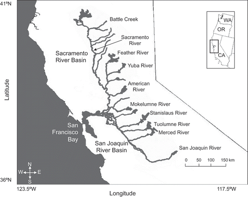
TABLE 1. Source hatcheries and fish facilities in California whose production and marking of Chinook Salmon contributed to this analysis. For the purposes of this report, we include Mokelumne River Hatchery among the Central Valley fall run but not the San Joaquin River basin fall run, since the Mokelumne River receives water and fish from the Sacramento River via the Delta Cross Channel. Start and end years refer to the earliest and latest brood years from which coded wire tags were recovered in the sport fishery and included in the size-at-age analysis (including harvest through 2010); these years do not necessarily coincide with the initiation or termination of hatchery production. In addition to the years listed, winter-run fish from Coleman National Fish Hatchery (NFH) were recovered from brood year 1978, and a small number of tags from natural-origin fish were recovered, including 60 Butte Creek spring-run tags in 1998–2004, 68 fall-run tags from the Yuba River in 1983–1987, 31 fall-run tags from the Feather River in 1997–2004, and 54 fall-run tags from the Mokelumne River in 1990–1999.
TABLE 2. List of hypotheses and predictions relating timing of life history events, ocean size, and maturation schedules of the different seasonal runs of Central Valley Chinook Salmon (WR = winter run; SR = spring run; FR = fall run; LFR = late-fall run).
FIGURE 2. Diagram showing the timing of key events in the life cycle of each Central Valley Chinook Salmon run, along with the aging convention used here (BY = brood year; OA = ocean age; SA = spawner age; PPR = peak parental return; PPS = peak parental spawning; JE = juvenile emergence; numbers denote ages; E/RP = emigration/release peak). Fingerling releases (as are typical) of the spring run are denoted by “(f)”; “ye” indicates the potential emigration of spring-run yearlings. Asterisks represent the return of spawning adults (with the number of asterisks indicating age); “ee” denotes the potential return of unusually early late-fall emigrants as age-1 spawners. Shading indicates the starting month for the comparison of ocean size at age or size at date. Italics indicate ages that are rarely observed.
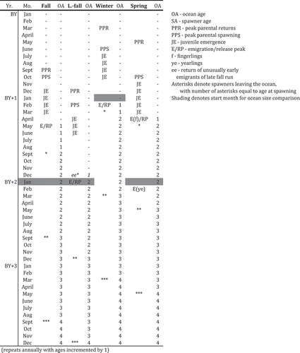
TABLE 3. List of variables used in this paper.
FIGURE 3. Monthly mean size (TL) at age for coded-wire-tagged Chinook Salmon recovered in the ocean for each Central Valley run. Circles are posterior medians; dotted lines are 68% credible intervals. In all cases, the x-axis starts with January of the calendar year following the end of the emergence period reported by Fisher (Citation1994). Arrows denote peak migration periods (adult return to freshwater) as identified by Fisher (Citation1994), labeled with the corresponding age at the subsequent spawning event, with arrows and numbers in gray for spawner ages that are rarely observed. Note that the spawning event may be separated from migration by an extended freshwater holding period and that migration timing can spread out over several months. For example, Vogel and Marine (Citation1991) report spring-run migration extending into early October. The timing of peak hatchery releases (see text) is denoted near the x-axis.
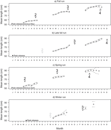
FIGURE 4. Monthly mean size (TL) at age for Sacramento River basin (black circles) versus San Joaquin River basin (gray squares) sourced fall-run Chinook Salmon recovered in the ocean. Points are posterior medians; dotted lines are 68% credible intervals.
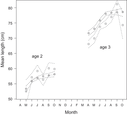
TABLE 4. Cumulative age structure (%) of tagged Chinook Salmon spawners returning to Central Valley hatcheries for each run (and for each basin within the fall run) for brood years 1998–2004 combined. The final column reports the sample size N (number of tags recovered). The diversity index is calculated as –1 times the sum over all age-classes of the proportion of spawners in that age-class times the natural logarithm of that proportion.
FIGURE 5. Age structure of returning spawners, by brood year, for Central Valley Chinook Salmon of the different run timings (and different basins for fall-run fish): (a) Sacramento River basin fall run; (b) San Joaquin River basin fall run; (c) late-fall run; (d) winter run; and (e) spring run. For each run, only brood years for which tagging, sampling, and reporting allowed for the possibility of recovering age-2 through age-4 fish are presented; this results in different temporal representation of the various runs. The dashed vertical line indicates the start of the 1998–2004 brood year period common to all stocks.
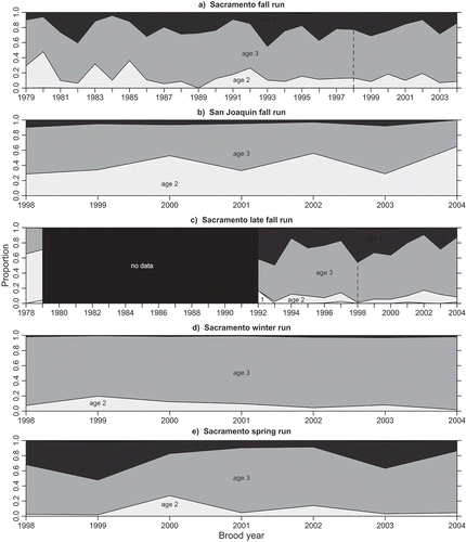
TABLE 5. Average (arithmetic mean) and SD of characteristics of hatchery releases for the various runs of Central Valley Chinook Salmon. Means were calculated by weighting the characteristics of different release groups by the number of fish from a release group recovered in the ocean fishery; therefore, these statistics do not summarize releases per se but instead summarize the characteristics of releases that contributed to the ocean harvest of coded-wire-tagged fish. The last two columns indicate the time from mean release until either the nominal peak of age-2 spawner returns (leaving the ocean; see ) or January 1 of the year after emergence (i.e., the reference time for ocean size comparisons). Sample sizes do not match total sample sizes for the size-at-age analysis because release characteristics were not reported for some releases.
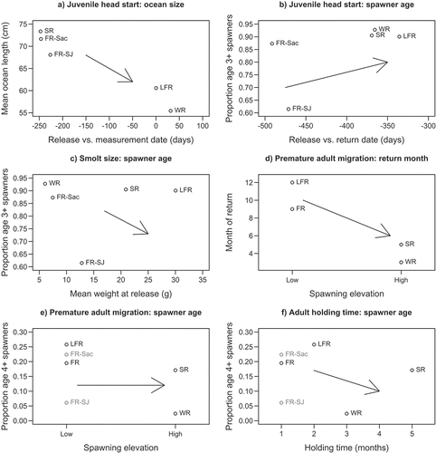
FIGURE 6. Graphical tests of hypotheses explaining variation among Chinook Salmon runs of the Central Valley (FR = fall run; LFR = late-fall run; SR = spring run; WR = winter run; Sac = Sacramento River basin; SJ = San Joaquin River basin). The juvenile head start hypothesis predicts that earlier entry to the ocean leads to (a) larger size at age/size at date and (b) earlier maturation of spawners. (c) The smolt size hypothesis predicts that larger smolts lead to earlier maturity. The premature adult migration hypothesis predicts (d) earlier return of stocks spawning further upstream but (e) no effect of spawning location on spawner age. (f) The adult holding time hypothesis predicts few large, old fish among stocks with extended holding time prior to spawning.