Figures & data
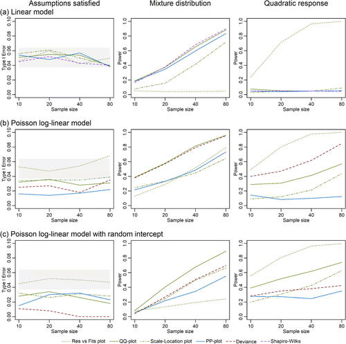
Fig. 1 Example diagnostic plots with global simulation envelopes, constructed using ecostats::plotenvelope, for the Salamanders data (Price et al. Citation2016) available in the glmmTMB package on R (Brooks et al. Citation2017). Three types of residual plot are presented: (a) a residual versus fitted values plot, (b) a QQ-plot, (c) a scale-location plot. A Poisson loglinear model with a random intercept was fitted using glmmTMB, and Pearson residuals computed from the fit. Global envelopes are the shaded areas, not that in (a) the envelope is so narrow that it is hardly visible. Note from (b) that many residuals on the QQ-plot fall outside their simulation envelope (taking unusually large values), and there is an increasing trend on the scale-location plot, which strays outside its envelope. Both of these trends are suggestive of overdispersion.
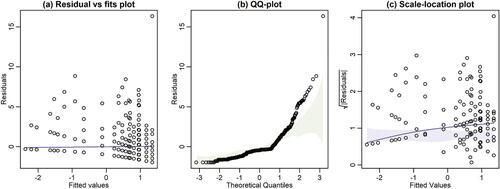
Fig. 2 Simulation results when fitting Models (a-c) to data simulated under the assumed model (left column), from a mixture distribution (center) or with a quadratic response to the predictor (right). In (a), the gray area is a 95% global envelope around the observed Type I error of an exact test, at significance level of 0.05, in this simulation design. Note in particular that all global simulation envelopes adequately control Type I error (left), that envelopes around QQ-plots (green solid line) were most effective at finding violations of distributional assumptions (center), and envelopes around a smoother on a residual versus fits plot (green dotted line) was most effective at finding violations of linearity (right).