Likelihood-Free Parameter Estimation with Neural Bayes Estimators

Figures & data

Fig. 1 Schematic of the DeepSets representation. Each independent replicate ${\mathit{Z}}_i$ is transformed independently using the function $\mathit{\psi }(·)$. The set of transformed inputs are then aggregated elementwise using a permutation-invariant function, $\mathit{a}(·)$, yielding the summary statistic T. Finally, the summary statistic is mapped to parameter estimates estimates $\widehat{\mathit{\theta }}$ by the function $\mathit{\varphi }(·)$. Many classical estimators take this form; in this work, we use neural networks to model $\mathit{\psi }(·)$ and $\mathit{\varphi }(·)$.

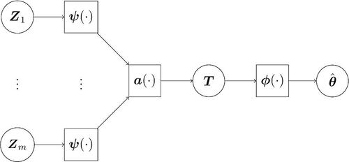
Fig. 2 Kernel density approximations to the distribution of the Bayes estimator (green line), our neural Bayes estimator (red line), the maximum likelihood estimator (purple line), and the one-at-a-time estimator (orange line), for θ from $\text{Unif}(0,\theta )$ data, where $\theta =4/3$ (gray dashed line) and where the sample size is m = 10.

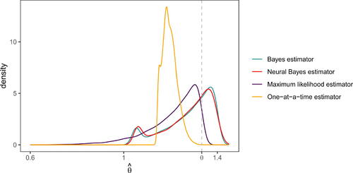
Fig. 3 The risk with respect to the 0–1 loss against the number of replicates, m, evaluated using the parameter vectors in the test parameter set, for the estimators considered in Section 3.2. The estimators ${\widehat{\mathit{\theta }}}_0(·)$, ${\widehat{\mathit{\theta }}}_{\text{DS}}(·)$, and the MAP estimator are shown in green, orange, and purple, respectively.

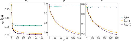
Fig. 4 The empirical joint distribution of the estimators considered in Section 3.2 for a single parameter vector. The true parameters are shown in red, while estimates from ${\widehat{\mathit{\theta }}}_0(·)$, ${\widehat{\mathit{\theta }}}_{\text{DS}}(·)$, and the MAP estimator are shown in green, orange, and purple, respectively. Each estimate was obtained from a simulated dataset of size $m=150$.

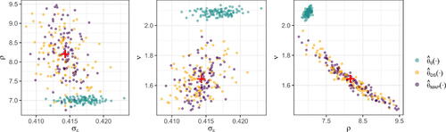
Fig. 5 Diagnostic plots for the simulation study of Section 3.3. (Left and center) The risk with respect to the 0–1 loss against the number of replicates, m, evaluated using the parameter vectors in the test parameter set. (Right) True parameters (red) and corresponding estimates, each of which was obtained using a simulated dataset of size m = 150. In all panels, ${\widehat{\mathit{\theta }}}_0(·)$, ${\widehat{\mathit{\theta }}}_{\text{DS}}(·)$, and the pairwise MAP estimator are shown in green, orange, and purple, respectively.

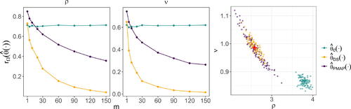
Fig. 6 The risk with respect to the 0–1 loss against the number of replicates, m, evaluated using the parameter vectors in the test parameter set, for the estimators considered in Section 3.4. The estimators ${\widehat{\mathit{\theta }}}_0(·)$ and ${\widehat{\mathit{\theta }}}_{\text{DS}}(·)$ are shown in green and orange, respectively.

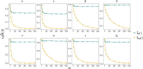
Fig. 7 (Lower triangle) The empirical joint distribution of the estimators considered in Section 3.4 for a single parameter vector. The true parameters are shown in red, while estimates from ${\widehat{\mathit{\theta }}}_0(·)$ and ${\widehat{\mathit{\theta }}}_{\text{DS}}(·)$ are shown in green and orange, respectively. Each estimate was obtained from a simulated dataset of size m = 150. (Upper triangle) Simulations from the model.

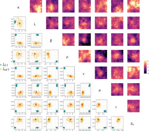
Table 1 Parameter estimates and 95% bootstrap confidence intervals (provided via the 2.5 and 97.5 percentiles of the bootstrap distribution) for the Red Sea dataset of Section 4.

	κ	λ	β	ρ	ν	μ	τ	δ1
Estimate	1.00	2.74	0.24	1.34	0.78	0.09	0.56	1.22
2.5%	0.88	2.13	0.14	0.95	0.70	0.04	0.49	0.91
97.5%	1.19	3.79	0.40	1.85	0.87	0.14	0.65	1.63

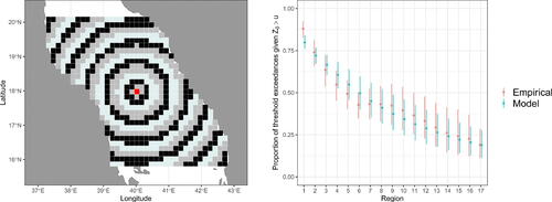
Fig. 8 (Left) The spatial domain of interest for the Red Sea study of Section 4, with the conditioning site, ${\mathit{s}}_0$, shown in red, and the remaining locations separated into 17 regions; the region labels begin at 1 in the center of the domain and increase with distance from the center. (Right) The estimated proportion of locations for which the process exceeds u given that it is exceeded at ${\mathit{s}}_0$ (points) and corresponding 95% confidence intervals (vertical segments) using model-simulated datasets (blue) and bootstrap samples of the observed dataset (red).