Trigonometric and cylindrical polynomials and their applications in electromagnetics

Figures & data

Figure 1. TP $L_{100}\left(x\right)=\sum _{m=1}^{100}\cos n_{m}x$, $x\in (0,\pi )$, with randomly distributed digits $1\le n_m\le 106$.

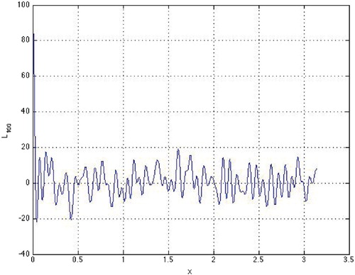
Figure 2. TPs $L_3\left(x\right)=\cos 3x+\cos 7x+\cos 20x$ (M=3, $n_{22}=7$, $n_{21}=3$, $n_3=20$) with $L_2\left(x\right)=\cos 3x+\cos 7x=2\cos 2x\cos 5x$, $x\in (0,\pi )$; $L_2\left(x\right)$ (o) has 7 zeros located together with 7 zeros of $L_3\left(x\right)$ (*) between pairs of neighboring zeros of $\cos 20x$.

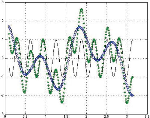
Figure 3. TPs $L_9\left(x\right)=\sum _{m=1}^9\cos n_{m}x$ (lower curve with greater number of oscillations) with ${\overline{\kappa }}_M=(n_1,\dots ,n_9)=(7,13,2,15,8,4,11,17,6)$, $L_8\left(x\right)=L_9\left(x\right)-\cos 6x$ (upper curve with greater number of oscillations), and $\cos 6x$, $x\in (0,\pi )$; zeros of TPs alternate and $L_9\left(x\right)$ and $L_8\left(x\right)$ have each 11 zeros located between pairs of neighboring zeros of $\cos 6x$.

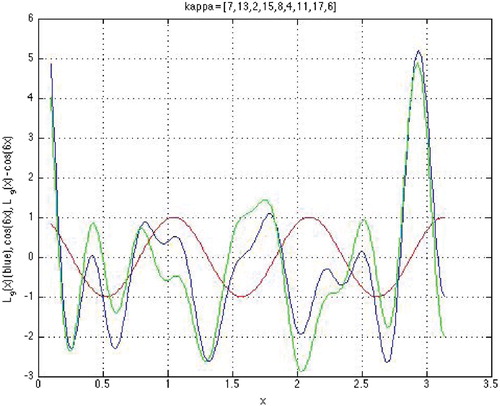
Figure 4. CPs $C_3\left(x\right)=J_0\left(3x\right)+J_0\left(7x\right)+J_0\left(20x\right)$ with $C_2\left(x\right)=J_0\left(3x\right)+J_0\left(7x\right)$, $x\in (0,\pi )$; $C_2\left(x\right)$ (o) has 4 zeros located together with 6 zeros of $C_3\left(x\right)$ (*) between pairs of neighboring zeros of $J_0\left(20x\right)$.

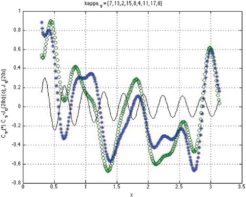
Figure 5. Zeros of a GCP $F_g$ (curve with highest oscillation) given by (21(21) $\begin{array}{r}{F}_g\left(x\right)\equiv P_D\left(qw\right){\mathrm{\Phi }}_1\left(x\right)-qx{\mathrm{\Phi }}_0\left(x\right)=0\left(\text{GL}\right),\end{array}$(21) ) situated between neighboring zeros of ${\mathrm{\Phi }}_0$ (curve with a negative starting value) and ${\mathrm{\Phi }}_1$ (curve with a positive starting value).

Figure 6. Example for a GCP $F_d\left(x\right)$ in DE (20(20) $\begin{array}{r}{F}_d\left(x\right)\equiv P_D\left(w\right)J_1\left(x\right)+x{J}_0\left(x\right)=0\left(\text{DW}\right),\end{array}$(20) ): plots of $J_0\left(x\right)$ (upper curve with no oscillations), $J_1\left(x\right)$ (lower curve with no oscillations), and $F_d\left(x\right)$ (curve with one oscillations) at $\epsilon =5$ and $\kappa =2$ ($u=\kappa \sqrt{\epsilon -1}=4$) displaying a zero of $F_d\left(x\right)$ between neighboring zeros of $J_1\left(x\right)$ and neighboring zeros of $J_0\left(x\right)$ and $J_1\left(x\right)$.

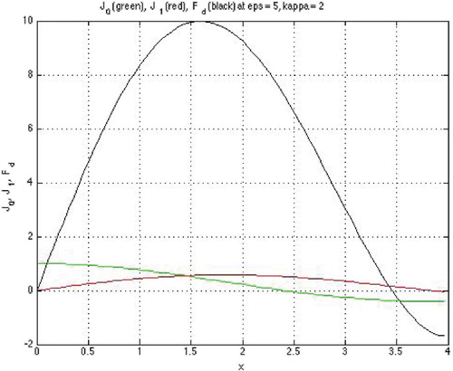
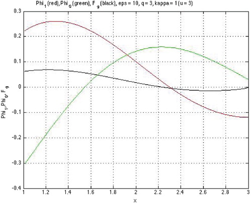
Figure 7. An example showing alternating zeros of ${\mathrm{\Phi }}_0\left(x\right)$ (curve starts at −0.3), ${\mathrm{\Phi }}_1\left(x\right)$ (curve starts above 0.2), and ${\mathcal{G}}_{2,4}^{\left(G\right)}=P_G{\mathrm{\Phi }}_0-{\mathrm{\Phi }}_1$ (curve starts above 0).