Solving a Cauchy problem for the heat equation using cubic smoothing splines

Figures & data

Figure 1. We illustrate the periodization process by displaying both a noisy data vector $f_{\mathrm{\Delta }}$ (left graph) representing a non-periodic function $f(t)$ defined on $[0,1]$. The cubic spline, defined on $[1,2]$ and that matches the slopes of $f(t)$ at t = 0 and t = 1 is also illustrated (left graph). The combined vector represents a periodic function defined on $[0,2]$. We also show the exact derivative $f^{\mathrm{\prime }}(t)$ (right graph) and the approximate derivative $D_{{\xi }_c}{f}_{\mathrm{\Delta }}$ for ${\xi }_c=35$ (right graph). The approximation is reasonably good both for t = 0 and t = 1.

Figure 2. We display the functions $f(t)$ and $h(t)$ in the top-left graph. In the top-right graph we show the error $\Vert f_{m,{\xi }_c}-f{\Vert }_2$, as a function of ${\xi }_c$, for the noise level $ϵ={10}^{-2}$. Note that there is an optimal value for ${\xi }_c$. In addition we display the solution $f_{m,{\xi }_c}(t)$, for ${\xi }_c=6$ (middle left), which is close to the optimum, and for ${\xi }_c=18$ (middle right). Also the exact solution $f(t)$ is displayed. In the bottom-left graph we show the optimal ${\xi }_c$ as a function of the noise level ϵ and in the bottom-right graph we show the corresponding error, for the optimal ${\xi }_c$, as a function of ϵ. Note that for a larger noise level ϵ, we need a smaller value of ${\xi }_c$, and obtain a larger error in the computed surface temperature $f_{m,{\xi }_c}(t)$.

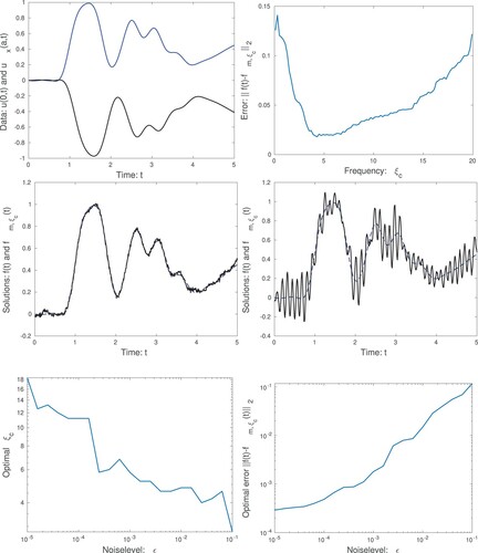
Figure 3. In the top-left graph we show the error $\Vert f_{m,\lambda }-f{\Vert }_2$, as a function of λ, for the noise level $ϵ={10}^{-2}$. Note that there is an optimal value for λ. In the top-right graph we display the surface temperature for $\lambda =2\cdot {10}^{-8}$ which is close to the optimal value. In the bottom-left graph we show the optimal λ as a function of the noise level ϵ and in the bottom-right graph we show the corresponding error, for the optimal λ, as a function of ϵ. Note that for a larger noise level ϵ, we need a larger value of λ, and obtain a larger error in the computed surface temperature $f_{m,\lambda }(t)$.

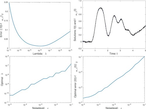
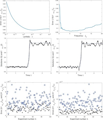
Figure 4. We present tests where the exact solution $f(t)$ is a smoothed step function. The top graphs show the error $\Vert f-f_{m,\lambda }{\Vert }_2$ (left) for the spline method and the error $\Vert f-f_{m,{\xi }_c}{\Vert }_2$ (right) for the Fourier method. The middle graphs display the numerical solutions $f_{m,\lambda }(t)$ (left) obtained using the spline method and $\lambda ={10}^{-8}$ and the solution $f_{m,{\xi }_c}(t)$ computed using the Fourier method and ${\xi }_c=7$. The lower graphs show the errors $\Vert f-f_{m_k,\lambda }{\Vert }_2$ x markers) and $\Vert f-f_{m_k,{\xi }_c}{\Vert }_2$ o markers) for different random noise sequences ${ϵ}_k$. In the left graph the variance of the noise is $ϵ={10}^{-2}$, $\lambda ={10}^{-8}$ and ${\xi }_c=7$. In the right graph instead $ϵ={10}^{-3}$, $\lambda =2\cdot {10}^{-9}$ and ${\xi }_c=8.3$. In both cases 100 different sets of random noise were generated.