Effect of trophic status of a deep-water lake on breeding Great Crested Grebes Podiceps cristatus during a phase of recovery from eutrophication: a long-term study

Figures & data

Figure 1. Total spring phosphorus in Lake Sempach 1965–2016.

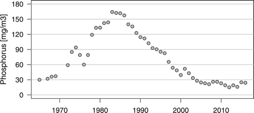
Table 1. Predictors used in the final models, with their mean, standard deviation and range of observed values. Predictors in italics were tested but not retained in the final models. GCG = Great Crested Grebes.

Parameter	Unit	Mean	Standard deviation	Range
Predictor variables:
Phosphorus	mg/m^3	38.5	23.1	15–90
Water transparency (Secchi disk depth)	m
April		3.02	1.51	1.70–7.00
May		2.98	1.28	1.20–5.80
June		3.50	1.15	1.50–6.50
July		2.93	0.84	1.40–4.70
August		2.94	1.00	1.20–4.80
Water level	m a.s.l.
May		503.809	0.156	503.6–504.1
June		503.839	0.164	503.5–504.1
July		503.800	0.121	503.6–504.1
Water temperature at depth of	°C
1.0 m		10.25	2.78	5.25–18.17
2.5 m		9.12	2.59	5.07–18.12
5.0 m		8.05	1.83	5.05–13.46
7.5 m		7.03	1.04	4.98–9.10
Rapid water level increase	no. of days with >5 cm	2.09	1.47	0–4
Strong wind (peak >70 km/h)	no. of days	2.30	1.52	0–5
between 1 June and 31 July
between 10 June and 15 July		1.26	1.14	0–4
Breeding pairs (predictor in models b and c)	n	281.1	87.4	118–436
National population index GCG	year 2000 = 1	0.93	0.14	0.73–1.27
European population index GCG
No. juveniles in preceding year
Zones with restricted access
Outcome variables:
Breeding pairs	n	281.1	87.4	118–436
Chicks per pair	n	0.63	0.27	0.23–1.28
Late broods	proportion	0.17	0.12	0.03–0.47

Table 2. Coefficient estimates for the final models of the three outcome variables. See Table 1 for explanations of the variables. Variables were z-transformed; an ‘x’ represents an interaction. All variables were in the a-priori defined models, except for the national population index in the first model which was added and retained based on its significance. In model b) strong wind 1 June to 31 July (estimate −0.10, P = 0.19) was replaced by the corresponding value for 10 June to 15 July; in all other cases, the month specified in the a-priori models was retained.

Coefficient	Estimate	se	t	P
a) Model for number of breeding pairs (quasi-Poisson model with log-link)
Intercept	5.44	0.04
Phosphorus, linear effect	−2.74	0.33	−8.2	<0.001
Phosphorus, quadratic effect	−0.95	0.28	−3.4	0.003
Water transparency in April	0.06	0.05	1.2	0.23
Water level in May	−0.05	0.04	−1.1	0.27
Water temperature in April at 1 m	−0.04	0.04	−1.1	0.27
National population index	0.14	0.04	3.5	0.003
b) Model for number of chicks per breeding pair (quasi-Poisson model with log-link and no. of breeding pairs as offset)
Intercept	−0.45	0.07
Phosphorus	0.29	0.10	2.8	0.01
Water transparency in June	0.12	0.07	1.7	0.10
Rapid water level increases	−0.02	0.07	−0.3	0.77
Strong winds, 15 June –15-July	−0.16	0.08	−2.0	0.07
Water temperature in April at 1 m	−0.01	0.08	−0.1	0.91
Rapid water level increase x Strong winds	0.05	0.08	0.6	0.53
c) Model for proportion of late broods (quasi-Poisson model with log-link and total no. families as offset)
Intercept	−1.91	0.12
Water transparency in June	−0.40	0.13	−3.0	0.009
Water level in June	−0.21	0.14	−1.5	0.15
Rapid water level increases	0.33	0.13	2.5	0.02
Strong winds, 1 June – 31 July	0.17	0.11	1.5	0.16
Water temperature	0.08	0.13	0.6	0.55
Rapid water level increase x Strong winds	0.00	0.13	0.0	0.98

Figure 2. Number of breeding pairs, number of chicks in late summer and reproductive success of Great Crested Grebes on Lake Sempach 1992–2016.

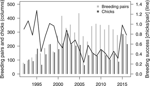
Figure 3. Partial effects of phosphorus (A) and national population index (B) on Great Crested Grebe population size in May. Circles indicate raw data, dotted lines the 95% confidence interval. Graphs show the effect of the parameter assuming constant values of the other parameters (set to their mean).

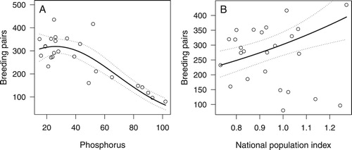
Figure 4. Partial effects of phosphorus (A), water transparency in June (Secchi disk depth) (B), and the number of days with strong wind 10 June to 15 July (C) on reproductive success of Great Crested Grebes (chicks/breeding pair).

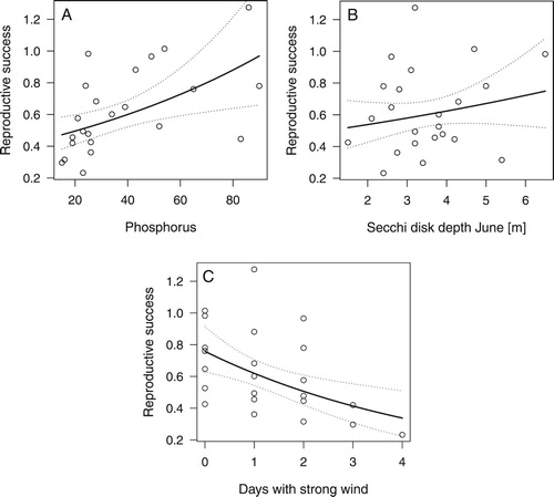
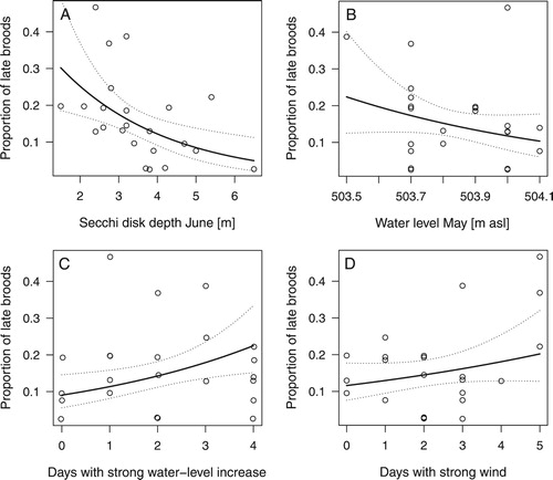
Figure 5. Partial effects of water transparency in June (A), water level in June (B), rapid water level increase (C), and number of days with strong wind (D) on the proportion of late broods of Great Crested Grebes.