Figures & data
Figure 1. Terrain and building facades as a canvas for portraying noise distribution (Pamanikabud and Tansatcha, Citation2010).
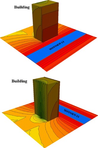
Figure 2. Noise visualization using building facades (Stoter et al., Citation2008).
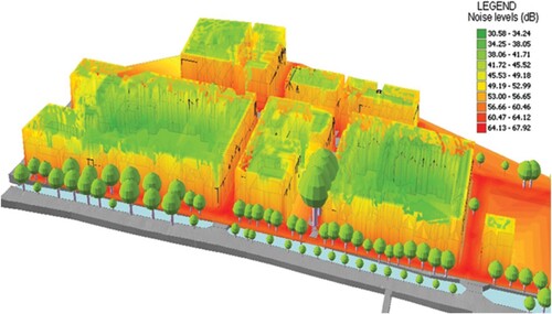
Figure 3. Noise visualization using cut by a vertical plane (Ranjbar et al., Citation2012).
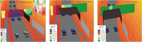
Figure 4. STC method used for continuous data (Fang and Lu, Citation2011).
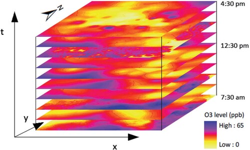
Figure 5. Types of data used for noise modelling, i.e. digital terrain model, 2.5D building models, 2.5D road networks and a 3D lattice of virtual microphones (four levels in Z dimension).
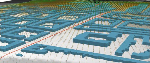
Figure 6. (a) 2D noise map, (b) Extruded building models and tilted observation angle, (c) Extruded building models and tilted observation angle with additional layers of noise for various heights.
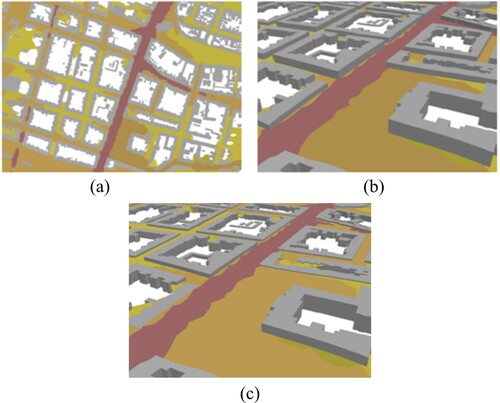
Figure 7. The scheme of the user experiment.
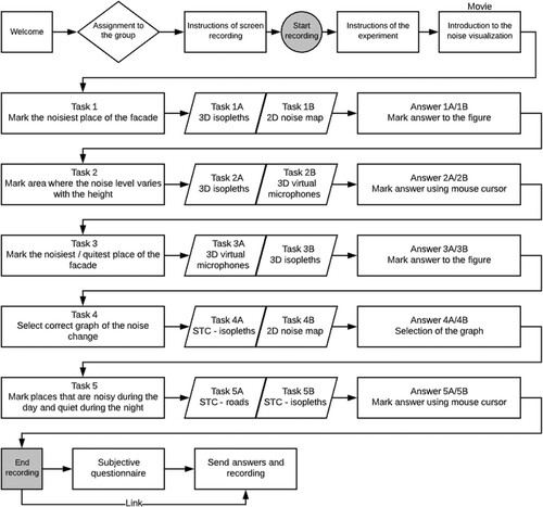
Figure 8. The user in image (a) was graded as correct since they accurately identified that the extreme noise levels occurring at the upper-left part of the façade; the user in the image (b) was partially correct (correct height, but not the specific part of the building), and the user in the image (c) was graded as incorrect.
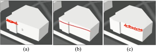
Table 1. Overview of presented methods, applications and user test tasks.
Figure 9. Noise levels with a minimum at 65 dB (red isopleth) (a) and noise levels with a minimum at 55 dB (orange isopleth) (b).
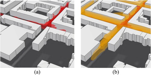
Figure 10. Difference in noise transmission with different noise barriers heights – noise levels affected by 3 m tall barrier (a), noise levels affected by 4 m tall barrier (b) and noise levels affected by 5 m tall barrier (c).
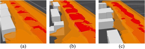
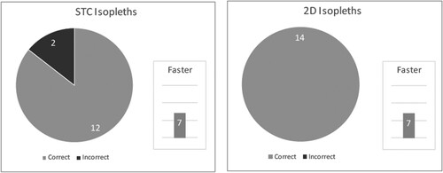
Figure 11. Task 1 user testing results – in the bar chart, see the number of faster participants using the corresponding visualization method. The pie chart shows the correctness of the answers.
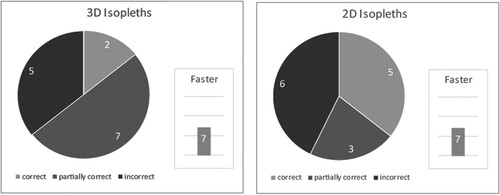
Figure 12. Virtual microphones spheres.
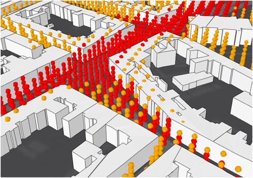
Figure 13. Task 2 user testing results.
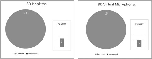
Figure 14. Task 3 user testing results.
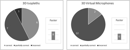
Figure 15. STC at traffic roads – only roads emitting over 75 dB (a), over 65 dB (b) and over 55 dB (c).
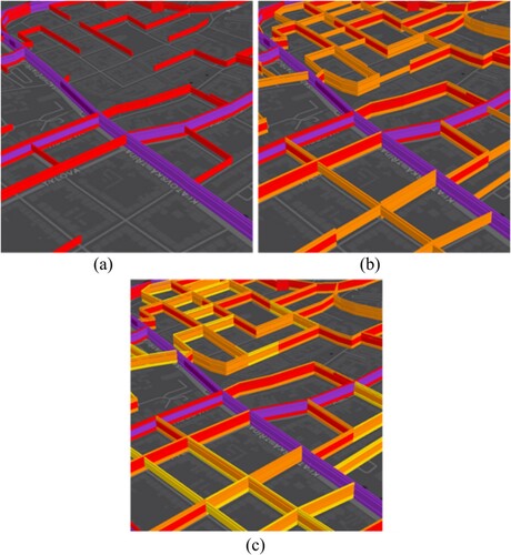
Figure 16. Task 4 user testing results.
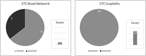
Figure 17. Correct answer to task 4 on the left (a) and example of an incorrect answer on the right (b).
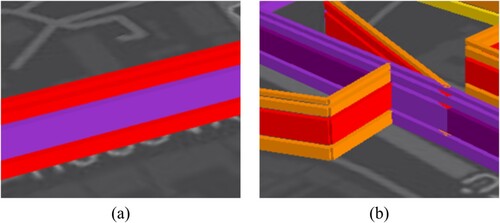
Figure 18. STC method with layers for different time intervals – (a) noise levels at a morning time interval (12 am–6 am), (b) morning and day time interval (6 am–6 pm), (c) morning, day and evening time interval (6 am–10 pm) and (d) morning, day, evening and night-time interval (10 pm–12 am).
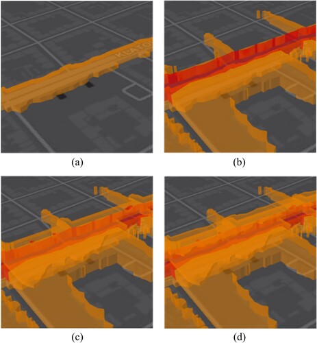
Figure 19. Task 5 user testing results.