Computing Data-driven Multilinear Metro Maps

Figures & data

Figure 1. Coordinate axes for different orientation systems. (c) illustrates a point p with the redundant coordinates $p=(0,1,\sqrt{2},1)$. (a) k = 2, irregular. (b) k = 3, regular aligned. (c) k = 4, regular rotated and (d) k = 5, regular rotated.

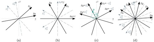
Figure 2. Illustration of how the slopes of the edges of a network (a) are interpreted as a set of circular data (b). Two distinct cases of clustering are shown in (c)–(e) and (f)–(h). We can cut the data (c) & (f) to obtain a 1-dimensional list of data points (d) & (g). After using a k-median clustering algorithm, we obtain an orientation system (e) & (h) from the median of every cluster. It is clear to see that the quality of the clustering is dependent on the choice of cut, e.g. $0^{\circ }$ in (c) or ${94}^{\circ }$ in (f). Note that our data range is only $0^{\circ }$ to ${180}^{\circ }$ and three points have been mirrored in (f) and (h) for illustrative purposes. (a) Example network. (b) Edge slopes. (c) Cut at $0^{\circ }$. (d) 1-dimensional data. (e) Resulting clustering. (f) Cut at ${94}^{\circ }$. (g) 1-dimensional data and (h) Resulting clustering.

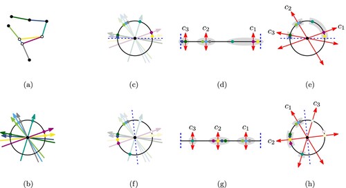
Figure 3. (a) For edges $(u,n_3),(u,n_0)$ the direction value decreases from 5 to 0. (b) The difference in angle between the orientations $z_0$ and $z_1$ (red arrow) is significantly smaller than between $z_1$ and $z_2$ (blue arrow). (a) Sector labeling and (b) k = 3, irregular.

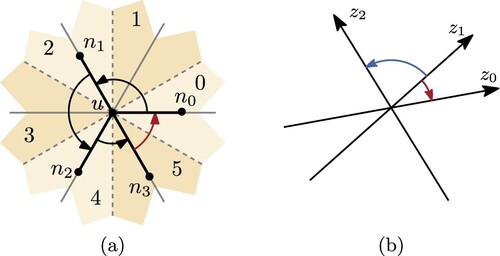
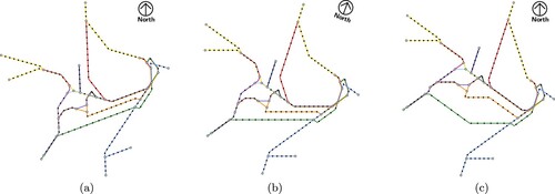
Figure 4. Examples of Sydney generated with objective function weights $(f_1,f_2,f_3)=(3,2,1)$ for different $k\in \{3,4,5\}$ and aligned (k-A), regular (k-R) and irregular (k-I) orientation systems. All shown instances reached the time-out limit of 1 h.

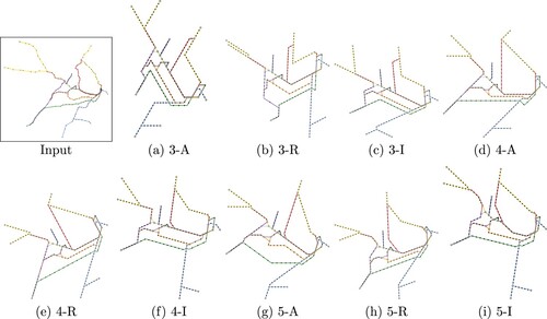
Figure 5. Plots of the results of the experiments for the objective function weights $(f_1,f_2,f_3)=(3,2,1)$. Every metric is shown as a coloured line, the columns are the three orientation systems.

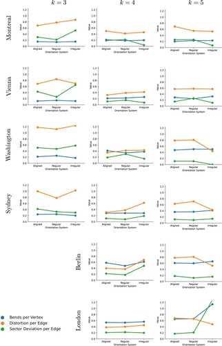
Table 1. Metric results for the Sydney network displaying the results for the different parameters, i.e. the number of available directions (k) and the orientation system (Aligned, Regular, Irregular).

	instance	Sydney
	linearity	k = 3			k = 4			k = 5
weights	orientation system	A	R	I	A	R	I	A	R	I
	bends	42.0	43.0	35.0	49.0	49.0	49.0	63.0	64.0	72.0
	sector deviation	41.0	32.0	29.0	11.0	8.0	18.0	12.0	10.0	14.0
	per edge	0.42	0.33	0.3	0.11	0.08	0.19	0.12	0.1	0.14
	distortion per edge	1.0	0.78	1.03	0.31	0.38	0.62	0.63	0.71	0.43
	time in seconds
$(3,2,1)$	optimality gap	0.2	0.2	0.16	0.13	0.12	0.1	0.11	0.08	0.07
	bends	31.0	32.0	35.0	48.0	47.0	47.0	59.0	59.0	59.0
	sector deviation	36.0	32.0	24.0	8.0	10.0	17.0	12.0	12.0	18.0
	per edge	0.37	0.33	0.25	0.08	0.1	0.18	0.12	0.12	0.19
	distortion per edge	0.88	0.84	1.02	0.29	0.33	0.59	0.65	0.68	0.49
	time in seconds									2216.0
$(10,5,1)$	optimality gap	0.09	0.07	0.05	0.01	0.02	0.01	0.01	0.01	0.0

Note: Metrics are the number of bends, sector deviation (total and per edge), distortion per edge (measured using ${\mathrm{dist}}_{\mathrm{\Delta }}\left(\mathcal{C}\right)$), the runtime in seconds (instances which reached the computation time limit of 1 h are marked with a clock symbol ) and the optimality gap in percent (listed as number between 0 and 1). For one set of objective function weights and linearity k combination the best value across all orientation systems of every metric is bold.

Figure 6. The transit network of Sydney using a 5-linear orientation system. (a) The computed angles of the regular orientation system (5-R) do not include a horizontal angle. (b) This map can be rotated until one direction coincides with the horizontal direction. The original north is indicated with a compass rose. (c) Note that, while the available directions are now the same as in the aligned map (5-A), they are oriented differently during the optimization and therefore the output maps are different. (a) Computed regular map (5-R). (b) Rotated regular map (5-R) and (c) Computed aligned map (5-A).