Figures & data
Figure 1. A schematic of variations of counted boxes at different box sizes to be used for the FDSGS approach.
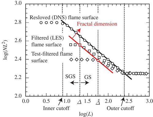
Figure 2. DNS configuration and simulated flame. Red iso-surfaces: , cyan iso-surfaces: the second invariant
.
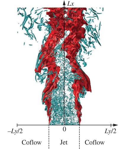
Figure 3. Inflowing (black) and local (red) turbulent combustion conditions in the combustion regime diagram (Peters, Citation2000). Arrows show trajectory along the streamwise direction.
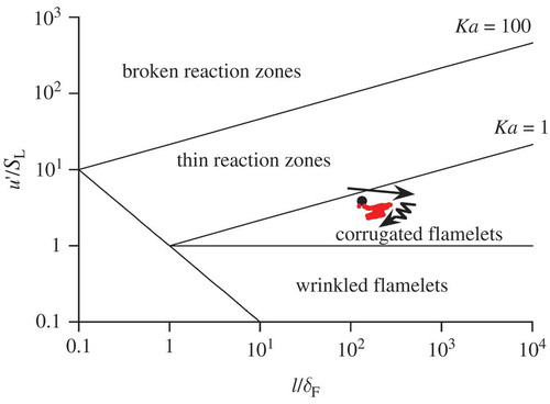
Figure 4. Streamwise development of the (a) fractal dimension and (b) the inner cutoff of flame surfaces using 3D and 2D box-counting methods.
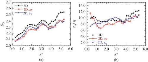
Figure 5. Dependence of the inner cutoff on . Lines: model values, and symbols: values from DNS and experiments.
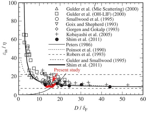
Figure 6. Temperature (in K) distribution on an instantaneous field obtained from the DNS of the turbulent jet premixed flame at . The flame surfaces represented by
contour are also shown.
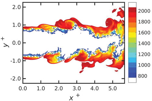
Figure 7. Streamwise development of the fractal dimensions of the flame surfaces obtained from the DNS data and predicted by the FDSGS combustion model with the Gaussian filters of (a) and (b)
.
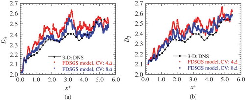
Figure 8. Streamwise distributions of Kolmogorov length scale obtained from the DNS data and computed using the FDSGS combustion model with the Gaussian filters.
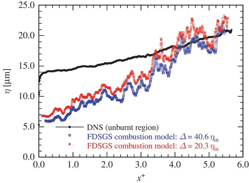
Figure 9. JPDFs of flame surface areas obtained from the DNS data and modeled using the FDSGS combustion model with the Gaussian filter of (a, c) and (b, d)
. The CV is set to be (a, b)
and (c, d)
. The black diagonal line represents the perfect agreement with the DNS results. The spacing of contour lines is logarithmically spaced by a factor of two.
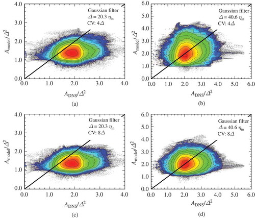
Figure 10. JPDFs of flame surface areas obtained from the DNS data and computed using several SGS combustion models of Colin et al. (Citation2000) (a, d), Flohr and Pitsch (Citation2000) (b, e), and Pitsch and Duchamp De Lageneste (Citation2002) (c, f) with the Gaussian filters of (top) and
(bottom).
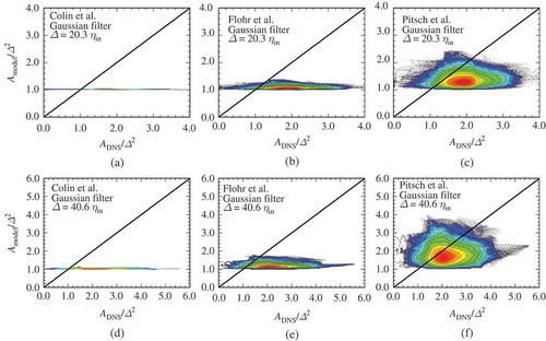
Table 1. Descriptions of conventional SGS combustion models compared in the present static tests.
Table 2. Conventional SGS combustion models considered in the present dynamic tests.
Table 3. Computational conditions of the LES and the DNS.
Figure 11. Instantaneous progress variable contours () in the spanwise mid-plane for DNS (gray line), LES11 (thin line), LES22 (dashed line), and LES43 (dashed-dotted line) with the FDSGS combustion model and CV size of
at (a)
and (b)
.
Figure 12. Mean temperature distributions in -direction for the filtered DNS data and results of LES11 (a, b), LES22 (c, d), and LES43 (e, f) at
(a, c, e) and
(b, d, f) in the case of
and
.
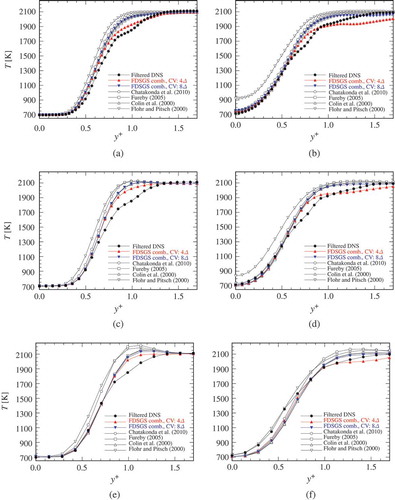
Figure 13. Variations of in
-direction for the filtered DNS data and results of LES11 (a, b), LES22 (c, d), and LES43 (e, f) at
(a, c, e) and
(b, d, f) in the case of
and
.
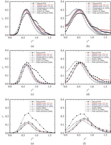
Figure 14. Transverse distributions of mean temperature (a) and RMS values of progress variable fluctuation (b) at for the filtered DNS data and LES22 simulated using the FDSGS combustion model. The size of CV is
and different Smagorinsky constants and turbulent Schmidt numbers as labeled are used.
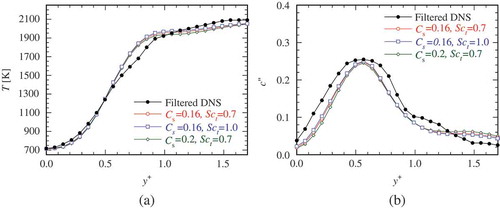
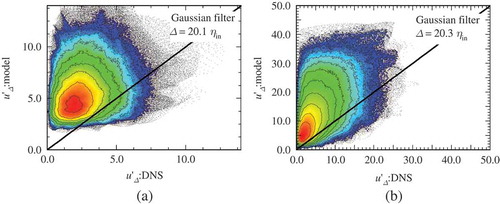
Figure 15. JPDFs of the SGS turbulent velocity fluctuations predicted by the Smagorinsky-type model (Flohr and Pitsch, Citation2000) and obtained from the DNS data for . Results for (a) turbulent planar premixed flame and (b) the present jet flame. Typical Smagorinsky constants are used:
for the planar case and
for the jet case.