Lean Flame Root Dynamics in a Gas Turbine Model Combustor

Figures & data

Figure 1. Schematic drawing of the gas turbine model combustor (Meier et al., 2006; Weigand et al., 2006).

Table 1. Operating conditions for flame C (Meier et al., 2006; Weigand et al., 2006).

Parameter	Value	Description
${\dot{m}}_{\mathrm{a}\mathrm{i}\mathrm{r}}$	$4.68\mathrm{g}/\mathrm{s}$	Air flow rate through the plenum
${\dot{m}}_{\mathrm{C}{\mathrm{H}}_4}$	$0.15\mathrm{g}/\mathrm{s}$	Methane flow rate through the nozzle
$P_{\mathrm{t}\mathrm{h}}$	$7.6\mathrm{k}\mathrm{W}$	Overall thermal power
$S$	$0.55$	Swirl number
ɸglob	$0.55$	Global equivalence ratio

Figure 2. Compuational grid for the gas turbine model combustor (a) and histograms of the normalised filter width distribution (b), where the cell samples are collected within the reaction region marked using $\overline{{\dot{\omega }}^{\ast }}>0$.

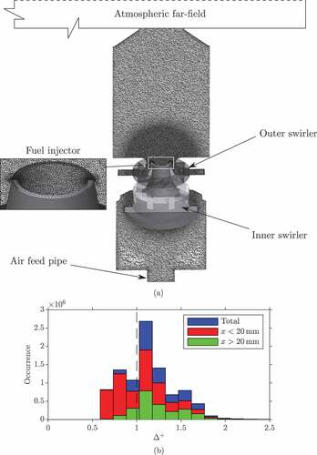
Figure 3. Distributions of the (a) axial velocity and (b) temperature fields for flame C. The filtered and averaged, in both time and the azimuthal direction, variations are shown on the left- and right-hand sides respectively. The corresponding streamlines are also shown.

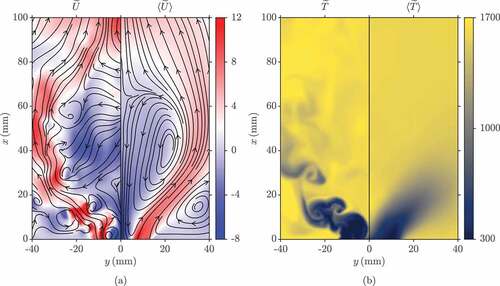
Figure 4. Comparisons of the time-averaged (a) axial and (b) radial and azimuthal velocities between the measurements (Meier et al., 2006; Weigand et al., 2006) (symbols) and the computations (lines), where the latter results are azimuthally averaged.

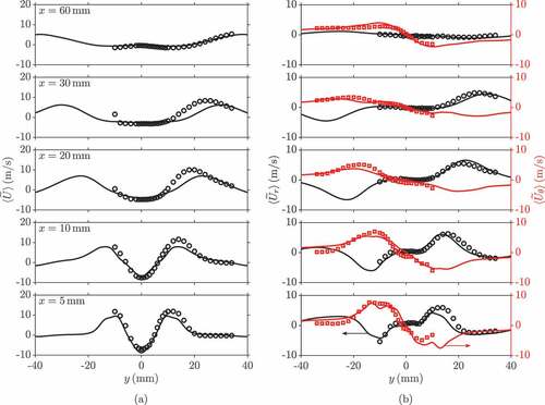
Figure 5. Comparisons of the time-averaged (a) axial and (b) radial and azimuthal rms velocities between the measurements (Meier et al., 2006; Weigand et al., 2006) (symbols) and the computations (lines), where the latter results are azimuthally averaged.

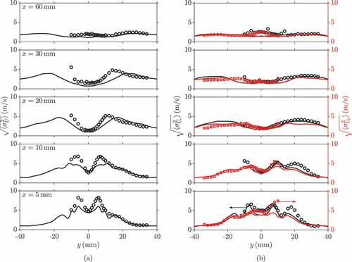
Figure 6. Comparisons of the time-averaged (a) mixture fraction and (b) temperature profiles between the measurements (Meier et al., 2006; Weigand et al., 2006) (symbols) and the computations (lines), where the latter results are azimuthally averaged.

Figure 7. Comparisons of the time-averaged (a) rms mixture fraction and (b) rms temperature profiles between the measurements (Meier et al., 2006; Weigand et al., 2006) (symbols) and the computations (lines), where the latter results are azimuthally averaged.

Figure 8. Distributions of the (a) filtered and (b) time-averaged heat release rate fields on the $x$–$y$ mid-plane.

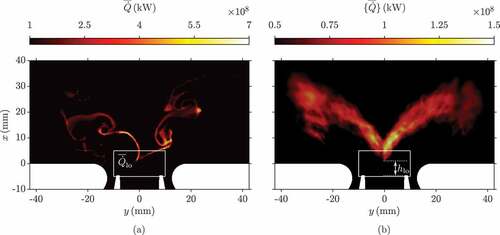
Figure 9. Time series of the (a) volume integrated heat release rate in the combustion chamber and within the marked volume in Figure 8 and (b) the lift-off height above the fuel nozzle.

Figure 10. Time series of the simultaneous (a) filtered reaction rate and velocity vectors (coloured by magnitude) and (b) PIV and OH–PLIF measurements for the flame in Stage 1.

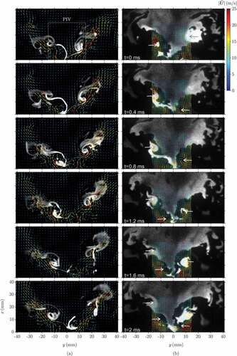
Figure 11. Time series of the simultaneous (a) filtered reaction rate and velocity arrows (coloured by magnitude) and (b) the PIV and OH–PLIF measurements for the event showing the loss of the flame root and local extinction.

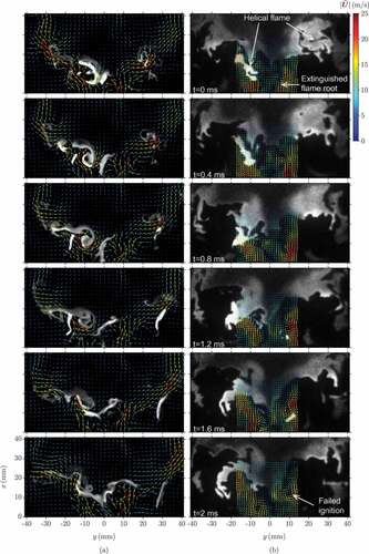
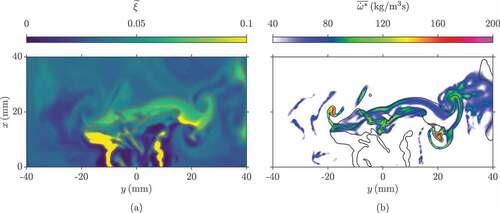
Figure 12. Distributions of the (a) filtered mixture fraction and (b) reaction rate for the flame in Stage 1 at t = 104.525 ms. The isolines denote the stoichiometric mixture fraction value of ${\xi }_{\mathrm{s}\mathrm{t}}=0.055$.

Figure 13. Distributions of the (a) filtered mixture fraction and (b) reaction rate prior to the lift-off event at $t=108.05\mathrm{m}\mathrm{s}$. The frames (c) and (d) respectively show the filtered mixture fraction and reaction rate at $t=111.05\mathrm{m}\mathrm{s}$.

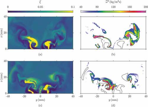
Figure 14. Distributions of the (a) filtered mixture fraction and (b) reaction rate for the flame at the maximum lift-off height ($t=138.5\mathrm{m}\mathrm{s}$).

Meier, W., Duan, X.R., and Weigand, P. 2006. Investigations of swirl flames in a gas turbine model combustor: II. Turbulence-chemistry interactions. Combust. Flame, 144(1–2), 225–236. doi:10.1016/j.combustflame.2005.07.009

 Web of Science ®Google Scholar

Weigand, P., Meier, W., Duan, X.R., Stricker, W., and Aigner, M. 2006. Investigations of swirl flames in a gas turbine model combustor: I. Flow field, structures, temperature, and species distributions. Combust. Flame, 144(1–2), 205–224. doi:10.1016/j.combustflame.2005.07.010

 Web of Science ®Google Scholar