Polydispersity Effects in Low-order Ignition Modeling of Jet Fuel Sprays

Figures & data

Figure 1. The modified Rosin-Rammler (a) accumulated volume and (b) droplet size pdfs in terms of $X$. The sauter mean diameter is shown in (b) for the range of $X$ highlighted in (a).

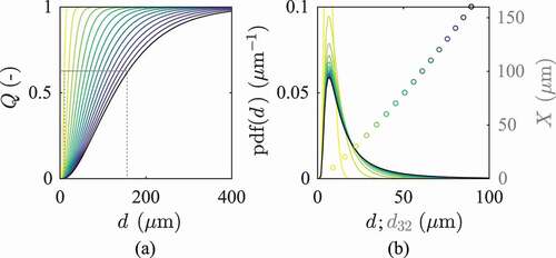
Figure 2. PDFs of the local equivalence ratio relative to the overall equivalence ratio in terms of the droplet distributions ($d_{32}=$ 20–90 mm) for cell size ${\mathrm{\Delta }}_x$ of 1.5, 3, and 5 mm – $\varphi =$ 0.7, $\mathrm{\Omega }=$ 0.

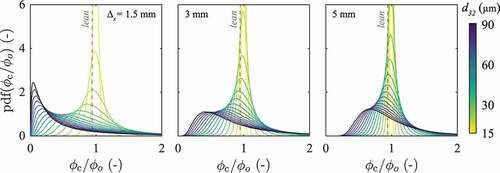
Figure 3. PDFs of the local equivalence ratio relative to the overall equivalence ratio in terms of the overall equivalence ratio $\varphi$ (0.4–3) for droplet distributions with $d_{32}$ of 15, 30, and 50 μm – ${\mathrm{\Delta }}_x=$ 3 mm, $\mathrm{\Omega }=$ 0.

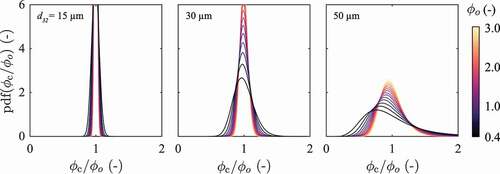
Figure 4. PDFs of the local equivalence ratio relative to the overall equivalence ratio in terms of the prevaporisation degree $\mathrm{\Omega }$ (0–0.95) for droplet distributions with $d_{32}$ of 30, 50, and 90 μm – $\varphi =$ 0.7, ${\mathrm{\Delta }}_x=$ 3 mm.

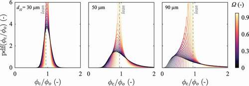
Figure 5. Flammability isosurfaces for cell sizes of (a) 1.5 and (b) 3 mm.

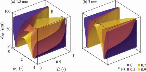
Figure 6. (a) Evolution of the number of burnt cells in the domain for $\mathrm{K}{\mathrm{a}}_{\mathrm{c}\mathrm{r}\mathrm{i}\mathrm{t}}$ set as 0.1, 0.3, 0.7, and 1. Ignition events are shown in gray and failed events in black. (b) Resulting probability of ignition for the conditions presented in (a) and comparison to experimental measurements – Jet A, ${\varphi }_{\mathrm{o}}=1$, ${\varphi }_{\mathrm{g}}=0.3$, $d_{32}=$ 29 μm (de Oliveira, Sitte, Mastorakos 2019).

Figure 7. Simultaneous (a) schlieren and (b) OH*-chemiluminescence of the spherically-expanding Jet A flames at 1 ms after the spark. The highest (33 μm) and lowest (16 μm) SMD conditions are shown for ${\varphi }_{\mathrm{o}}=1$ and 1.4. Modified from de Oliveira and Mastorakos 2019.

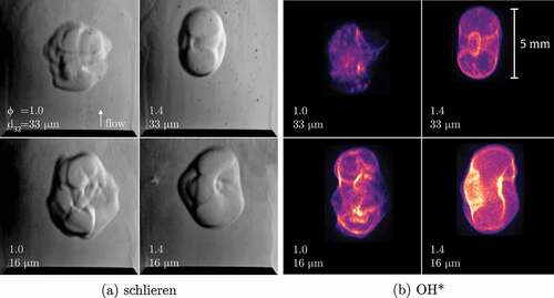
Figure 8. (a) Calibrated critical Karlovitz number for Jet A and (b) comparison of flame speed measurements de Oliveira and Mastorakos (2019) and values obtained with the correlation by Neophytou and Mastorakos (2009).

Figure 9. Comparison between simulations with and without liquid fuel fluctuation. (a) An example of the calibration for a single condition (Jet A, ${\varphi }_o$= 1.4, $d_{32}=$33 μm). (b) The resulting calibration for all conditions.

de Oliveira, P. M., M. P. Sitte, and E. Mastorakos (2019), Validation of a low-order model for ignition of sprays. AIAA Scitech 2019 Forum, Reston, Virginia, American Institute of Aeronautics and Astro- nautics

 Google Scholar

de Oliveira, P. M., and E. Mastorakos. 2019. Mechanisms of flame propagation in jet fuel sprays as revealed by OH/fuel planar laser-induced fluorescence and OH* chemiluminescence. Combust. Flame. 206:308–21. doi:https://doi.org/10.1016/j.combustflame.2019.05.005.

 Web of Science ®Google Scholar

Neophytou, A., and E. Mastorakos. 2009. Simulations of laminar flame propagation in droplet mists. Combust. Flame. 156 (8):1627–40. doi:https://doi.org/10.1016/j.combustflame.2009.02.014.

 Web of Science ®Google Scholar