Figures & data
Table 1. Details of the operating conditions and geometric parameters for the simulated cases; SOI: Start of injection, EOI, End of injection, : In cylinder air to fuel ratio, CO
ratio: ratio between in cylinder CO
and stoichiometric CO
Figure 1. Geometry of the engine and the mesh used in the study.
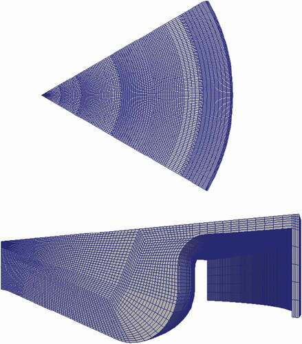
Table 2. Description of different numerical cases. HL: High Load, LL: Low Load, S: Swirl Number, SOI: start of injection, : injection pressure. The ones marked with EXP are the points where the experimental data are available
Figure 2. Pressure trace for different cases at high load.
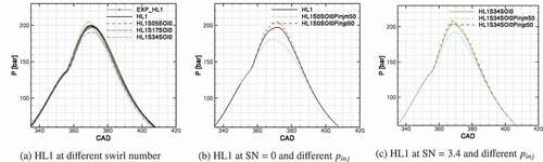
Figure 3. In-cylinder soot mass for different cases at high load.
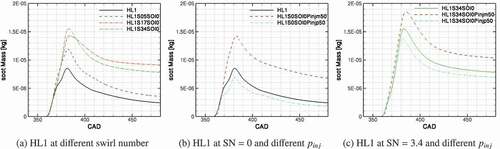
Figure 4. Variation of lean, flammable, and rich mixture inside the cylinder.
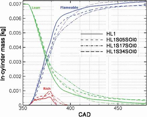
Figure 5. Apparent rate of heat release and injection profile for the high load case 1.
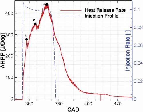
Figure 6. In-cylinder temperature field at different combustion events.
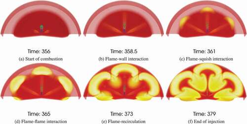
Figure 7. Formation, oxidation and net rate of soot for the HL1 case. The injection profile and total in-cylinder soot mass are presented for comparison.
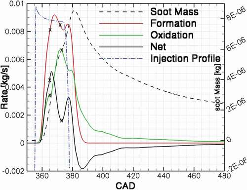
Figure 8. Left: Combustion duration for different swirl ratio and injection pressure, right: Soot mass at the end of combustion for different swirl ratio and injection pressure.
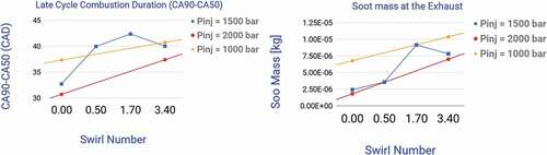
Figure 9. Rate of heat release for different swirl ratios.
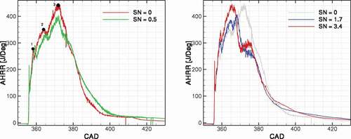
Figure 10. From left, 2D contour of heat release rate with line contour of mixture fraction (Z), vorticity in the Z direction, formation rate of soot volume fraction and production term of turbulent kinetic energy for the no swirl case. Moving Plane A is used.
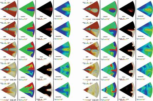
Figure 11. Formation, oxidation and net rate of soot at different swirl ratios.
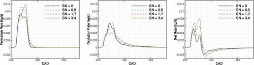
Figure 12. a) Scatter plot of soot emissions and half-life time of soot as a representative of soot oxidation process and b) scatter plot of peak value of soot and soot emission as a representative of soot formation process.
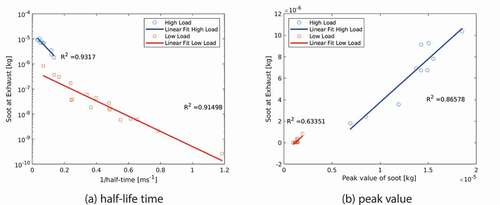
Figure 13. Planes where the numerical data are extracted. from left, first, plane I in the middle of the spray axis parallel with the cylinder fire deck. Second, plane II, in the middle of the spray with the angel of 30 degree with the cylinder head. Third, Moving Plane A in the middle of the bowl with the normal in the Z direction, and fourth, Moving Plane B right above the piston bowl with the normal in the Z direction.
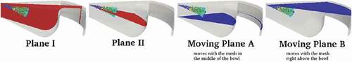
Figure 14. Structure of the flow inside the cylinder at planes I and II for the four swirl numbers, SN = 0, 0.5, 1.7 and 3.4. Velocity vectors are colored with O mass fraction and the 2D contours represent the soot volume fraction.
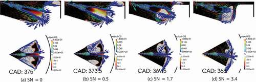
Figure 15. Structure of the flow inside the cylinder at planes I and II for the four swirl numbers, SN = 0, 0.5, 1.7 and 3.4. Velocity vectors are colored with O mass fraction and the 2D contours represent the soot volume fraction.
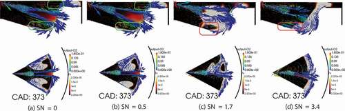
Figure 16. Flow streamlines and soot volume fraction and soot oxidation contours at Moving Plane B at CAD 370 to 380.
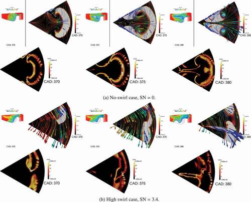
Figure 17. Structure of the flow inside the cylinder at planes I and II for SN = 0 and 3.4. Velocity vectors are colored with O mass fraction and the 2D contours represent the soot volume fraction.
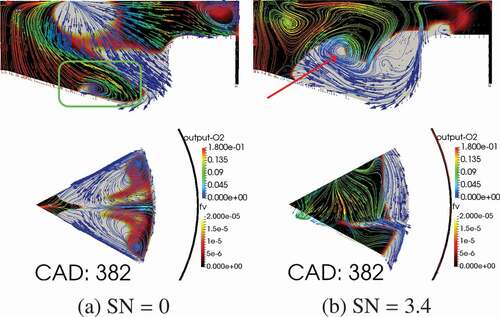
Figure 18. Structure of the flow inside the cylinder at planes I and II for the no-swirl case, SN = 0. Velocity vectors are colored with O mass fraction and the 2D contours represent the soot volume fraction.
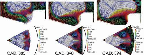
Figure 19. Structure of the flow inside the cylinder at planes I and II for the high swirl case, SN = 3.4. Velocity vectors are colored with O mass fraction and the 2D contours represent the soot volume fraction.
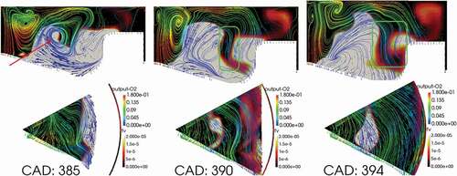
Figure 20. Kinetic energy, turbulent kinetic energy for different swirl numbers and swirl ratio history of the high swirl case.
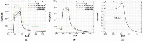
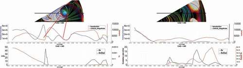
Figure 21. Production term of turbulent kinetic energy, vorticity magnitude, soot, and soot oxidation rates across a vortex structure in Moving Plane B at CAD 375.
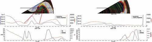
Figure 22. Production term of turbulent kinetic energy, vorticity magnitude, soot, and soot oxidation rates across a vortex structure in Moving Plane B at CAD 380.