Figures & data
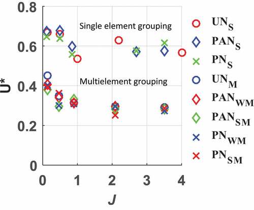
Figure 1. Assembly drawing of the combustion chamber.
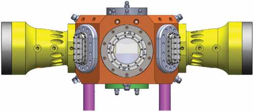
Figure 2. Schematic of the inner channel inside the pressure containment.
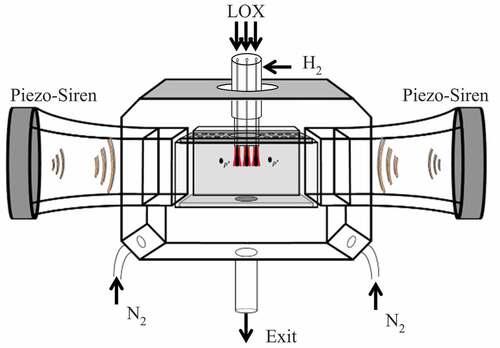
Figure 3. The injector faceplate for: (a) the single element and (b) the multi-element. The injectors are in green (LOX) and red (GH2). The gray is the solid injector support. The black external to the gray is GN2 for recirculation suppression (solid circles) and window cooling (linear slots).
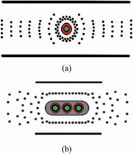
Figure 4. High speed, simultaneous shadowgraph and OH* imaging system.
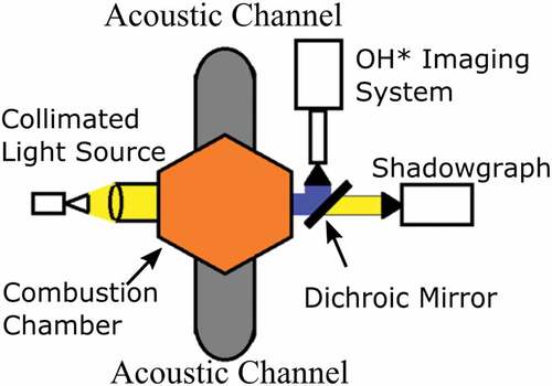
Table 1. Flow conditions. First/second cell entries: acoustic (this paper)/non-acoustic (previous paper) values.
Table 2. Acoustic conditions (this paper). First/second cell entries: weak/strong acoustic amplitudes.
Figure 5. Differential pressure measurements of the three window pressure transducers for strong forcing: (a) PAN and (b) PN.
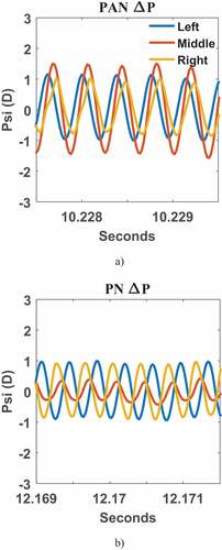
Figure 6. PSDs of the differential pressure signal at the forcing frequency (a) PAN and (b) PN.
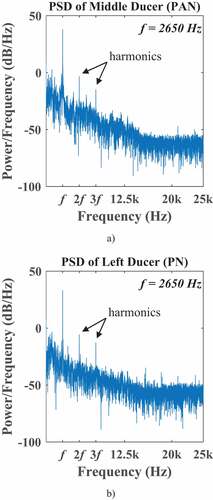
Figure 7. Example of a standing wave reconstructed from the pressure measurements. (a) pressure antinode (velocity node). (b) pressure node (velocity anti-node).
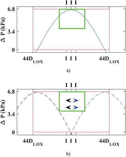
Figure 8. Full temporal averages of the multi-element shadowgraph and OH* emissions under strong PAN (left columns) and strong PN (right columns) forcing.
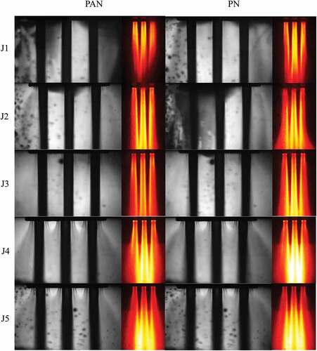
Figure 9. Instantaneous images of the multi-element shadowgraph and OH* emissions under strong PAN (left columns) and strong PN (right columns) forcing.
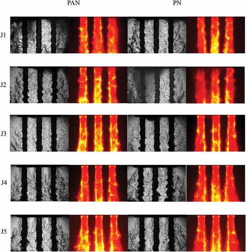
Figure 10. Phase-averaged images of the multi-element shadowgraph and OH* emissions under strong PAN (left columns) and PN (right columns) forcing. The white lines indicate the downward, outward slanting discussed in the text.
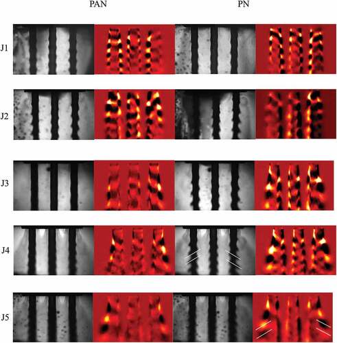
Figure 11. Nesting modes. (a) varicose (out-of-phase). (b) sinuous (in-phase), (c) varicose (in-phase, destructive). Not illustrated, except for the collisional breakdown in (c), is the eventual downstream dissipation of all modes by the background turbulence.
Figure 12. Interrogation windows for CPSD (small green boxes) and DMD (large yellow box).
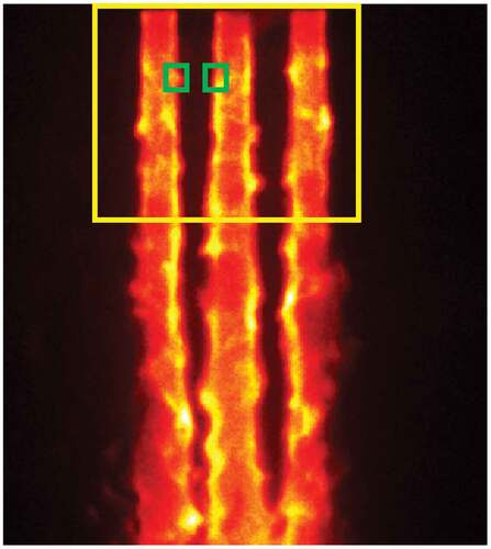
Figure 13. Phases from a CPSD analysis of the OH* images between the left and center flames at the natural frequencies (a), or at the forcing frequencies (b,c), as a function of J. A positive phase angle indicates the center flame leads in time: (a) unforced, (b) PAN, and (c) PN.
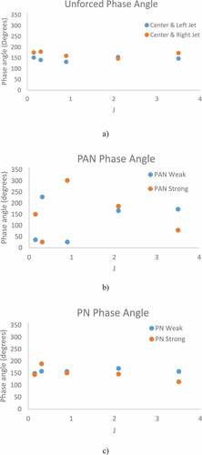
Figure 14. OH* emission DMD spectra as a function of J for the weak PAN and PN (left two columns), and the strong PAN and PN (right two columns).
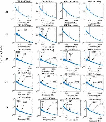
Table 3. Weak PN frequencies.
Figure 15. DMD spatial modes at the natural frequencies for weak forcing.
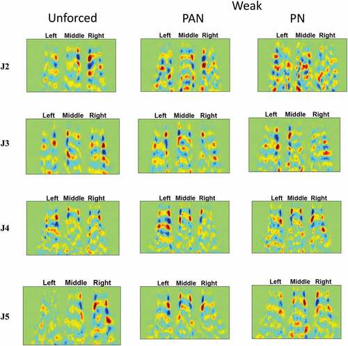
Figure 16. DMD modes at the peak frequencies for J2 at a weak PN. (a) low (difference) frequency mode, (b) driving frequency mode, (c) high (natural) frequency mode.
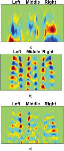
Figure 17. OH* emission DMD spatial modes at the forcing frequencies. The left two columns are for the weak PAN and PN, and the right two columns are for the strong PAN and PN.
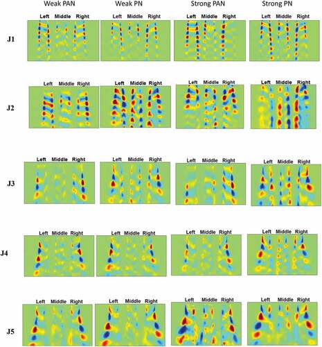
Figure 18. Average OH* wave velocities of the center flame, normalized by the mean of the propellant bulk velocities (U*, Equationeq. 1)(1)
(1) . Symbols in the legend are as follows: PAN – pressure antinode, PN – pressure node, UN – unforced. The meanings of the subscripts in the legend are: S – single element, M – multielement (unforced), WM – multielement (weak forcing), SM – multielement (strong forcing).