Characterization of Flame Spread Over PMMA Using a Temperature Reconstruction Method

Figures & data

Figure 1. Regimes of opposed flow spread: downward, horizontal, and lateral spread.

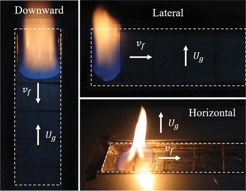
Figure 2. Middle: A schematic representation of the relevant heat transfer mechanisms dictating opposed flow flame spread. Left: A representation of the relevant gas phase heat transfer (both gas phase conduction and radiation). Right: a representation of conduction through the solid phase ahead of the flame front.

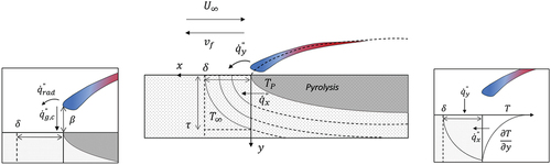
Figure 3. Flame spread rates for each configuration determined using both video analysis and surface temperature measurements considering all measurement locations and repeat trials. Video data was averaged across repeat trials and was only analyzed between 30–170 mm.

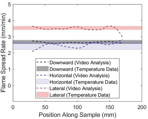
Figure 4. The time histories of temperature measurements at each measurement location along the sample as the flame front approached. The consistent time histories observed as the flame front approaches each location indicates steady flame spread behavior. Data presented for downward flame spread. All x positions are presented in mm.

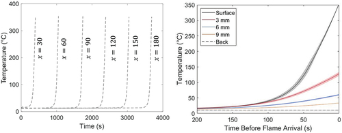
Figure 5. A graphical explanation of the temperature reconstruction method used in this study.

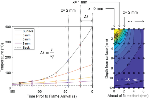
Figure 6. Simulated thermal distributions in the solid ahead of the flame front determined using the temperature reconstruction method. Distributions simulated for downward (left), horizontal (middle), and lateral (right) spread. All contours in °C.

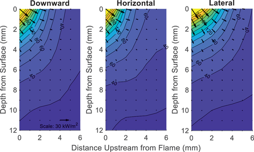
Figure 7. Top figures: the thermal gradients ahead of the flame front in both the x and y direction. These gradients are then evaluated at either x=0 or y=0 for each depth or position along the surface, through which the conductive (${\dot{q}}_x^{{ }^{\prime \prime }}$) and gas phase (${\dot{q}}_y^{{ }^{\prime \prime }}$) heat transfer rates can be calculated (lower figures).

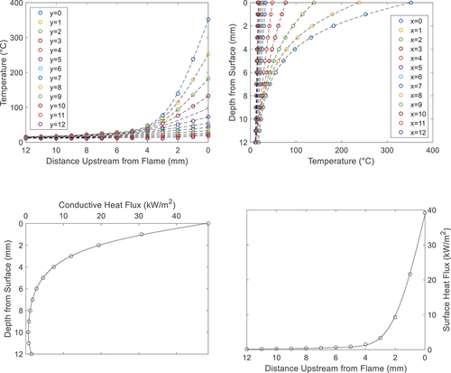
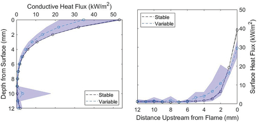
Figure 8. A comparison of the conductive heat flux distribution (${\dot{q}}_x^{{ }^{\prime \prime }}$) and the gas phase heat flux distributions (${\dot{q}}_y^{{ }^{\prime \prime }}$) across the three configurations used in this study.

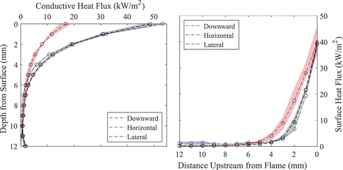
Table 1. Resulting flame spread rates, heat flux contributions, and relevant characteristic length scales as defined by Equations 1(1) ${{\dot{q}}_x}^{\prime \prime }=k_s{\left.\frac{\mathrm{\partial }{T}_s}{\mathrm{\partial }x}\right|}_{x=0}$(1) –4(4) ${{\dot{q}}_{l,surf}}^{\prime \prime }=\epsilon \sigma \left(T_{surf}^4-T_{\mathrm{\infty }}^4\right)$(4) .

Configuration	${\mathit{v}}_{\mathit{f}}$ (mm/min)	$\dot{{\mathbf{Q}}^{\prime }}x$ (W/m)	${\dot{\mathit{Q}}}_y^{\prime }$ (W/m)	${\dot{q}}_{f}2\delta$δ (kW^2/m)	Max ${{\dot{q}}^{″}}_y$ (kW/m^2)	Max ${\dot{\mathit{q}}}_{\mathit{x}}^{{ }^{\prime \prime }}$ (kW/m^2)	δ (mm)	τ (mm)
Downward	2.67 $\pm$ 0.13	106	57	1.23	41.2	50.6	3.6	6.4
Horizontal	2.54 $\pm$ 0.50	101	58	1.08	40.4	54.7	3.4	5.3
Lateral	3.54 $\pm$ 0.17	45	82	1.91	46.1	18.9	5.0	6.5

Figure A1. A schematic representation of the thermocouple placement within each sample tested. At each location, three in-depth measurements were made in addition to a surface temperature measurement. Back face temperatures were measured from the temperatures recorded for the water cooling system. All dimensions in mm.

Figure A2. The water-cooled sample holder used in this study. Continuous water cooling was provided through the four holes passing through the length of the sample holder. Additional holes were milled through the sides of the sample holder to insert the thermocouples in-depth within the solid.

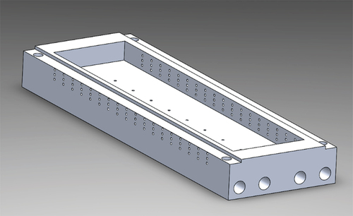
Figure B1. Temperature time histories as the flame approaches each station for a horizontal flame spread trial. The first two stations display stable temperature readings (solid lines), while the remaining stations display a different heating behavior (dashed lines).

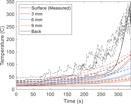
Figure B2. A comparison on the gas phase and conductive heat fluxes calculated for the stable temperature readings seen in Figure and the variable readings seen as the flame grows more turbulent.