A simple recipe to calculate the thermal conductivity of anharmonic crystals: the case of SrTiO₃

Figures & data

Figure 1. (a) The phonon dispersion of the lowest transverse optic (squares) and acoustic (circles) modes of STO along (100) as a function of temperature; the inset to the figure shows the squared of the soft ferroelectric mode ${\omega }_{TO}^2(q=0)$ as a function of temperature (black line and symbols) in comparison to experimental data (blue and green stars) from Refs. [49,50]; (b) the difference between the transverse optic (TO) and transverse acoustic (TA) mode frequencies as a function of momentum q and temperature. The inset to this figured shows the phonon mean free path which is derived from the minimum in Δ(ω) = ω_TO(q) − ω_TA(q), where the inverse of the crossing momentum of optic and acoustic modes defines the mean free path $l_{ph}$ which is identical for both modes.

Figure 2. Group velocities of the optic v_TO and the acoustic v_TA modes as a function of momentum q and temperature.

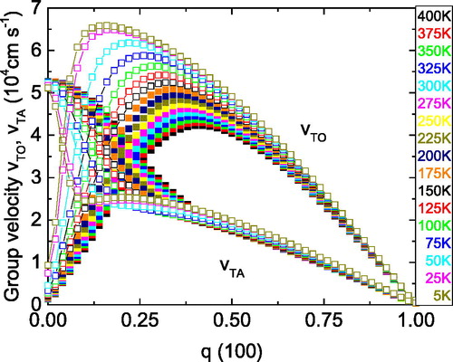
Figure 3. (a) v_TO in the limit q → 0 as a function of temperature, (b) the same as (a) but for v_TA. The squares and circles refer to the calculations, the full lines are obtained from an exponential fit to the calculation. Note, that the scale of the y-axis is different in both figures.

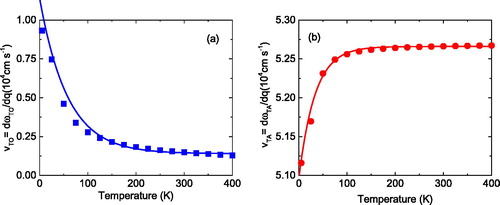
Figure 4. The specific heat c_V of STO as a function of temperature in comparison to experimental data (red open circles). The inset shows the derivative with respect to temperature of c_V as a function of temperature again in comparison with the experimental data (red open circles).

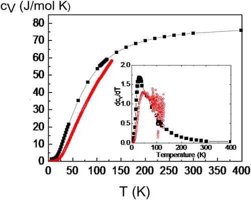
Figure 5. TC as a function of temperature for STO shown on a double logarithmic scale. The experimental data of Ref. [12] of STO are represented by the black squares. The theoretically obtained results are given by the red squares.

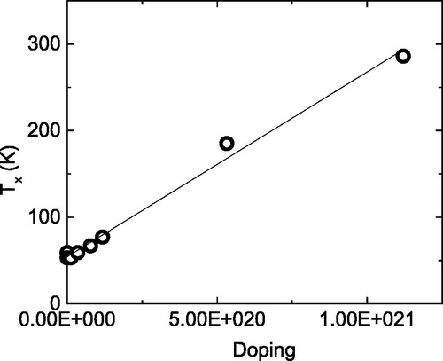
Figure 6. The characteristic temperature scale T_x as a function of doping.

J. Petzelt et al., Dielectric, infrared, and Raman response of undoped SrTiO3 ceramics: evidence of polar grain boundaries, Phys. Rev. B. 64 (18), 184111 (2001).

 Web of Science ®Google Scholar

J. L. Servoin, Y. Luspin, and F. Gervais, Infrared dispersion in SrTiO3 at high temperature, Phys. Rev. B. 22 (11), 5501 (1980). DOI: 10.1103/PhysRevB.22.5501.

 Web of Science ®Google Scholar

V. Martelli et al., Thermal transport and phonon hydrodynamics in strontium titanate, Phys. Rev. Lett. 120 (12), 125901 (2018).

 PubMed Web of Science ®Google Scholar