Reports of Value’s Death May Be Greatly Exaggerated

Figures & data

Table 1. Major Factor Performance, US Stocks

		July 1963–June 2020					January 2007–June 2020
Factor	Year of Discovery	Average Return	St. Dev.	t-Stat.	CAPM α t-Stat.		Average Return	St. Dev.	t-Stat.	CAPM α t-Stat.
Market	1964	6.5%	15.4%	3.17			8.6%	15.9%	1.99
Value	1977–90	3.0	9.8	2.34	3.12		–5.4	9.9	–2.00	–2.64
Size	1975	2.2	10.3	1.63	0.70		0.0	8.0	–0.01	–0.83
Profitability	2013	2.8	7.7	2.77	3.55		3.2	5.6	2.08	2.81
Investment	2003	2.5	6.3	3.00	4.36		–0.6	4.8	–0.48	–0.38
Momentum	1989	7.8	14.5	4.04	4.57		1.2	16.4	0.27	1.13
Low beta	1966	0.2	15.4	0.10	3.47		–2.7	16.4	–0.62	1.22

Notes: All returns are for long–short strategies based on factors (similar to the HML factor of Fama and French). Reported are both the t-statistics for the return of the long–short portfolios and the t-statistics for the corresponding CAPM alphas. Because the capital asset pricing model (CAPM) adjusts for market risk and given that many of the factors had negative market betas in the 1963–2020 period, the t-statistics associated with CAPM alphas tend to be higher than those for simple returns. The adjustment for market risk is particularly important for the low-beta factor. This factor’s average return is close to zero, but given its negative market beta, it has a statistically significant CAPM alpha. The long–short factor has a negative market beta because the long side contains stocks with below-1.0 market betas and the short side contains stocks with above-1.0 market betas. We used the Fama and French (2015) definition for the investment and profitability factors (where the profitability factor was initially popularized by Novy-Marx 2013). We also followed the definition of the momentum factor from the website of Kenneth French: https://mba.tuck.dartmouth.edu/pages/faculty/ken.french/data_library.html. The momentum factor was first documented by Jegadeesh and Titman 1993; it was popularized by Asness 1994 and Carhart 1997 as part of factor models.

Sources: Research Affiliates, LLC, using data from CRSP/Compustat.

Table 2. US Value Stocks vs. US Growth Stocks: Worst Value Drawdowns, July 1963–June 2020

		Dates
Rank	Event	Start Date	Bottom	End Date	Length	Drawdown
A. Deepest drawdowns
1	Current	2006/12	2020/06	—	13 yrs., 6 mos.	–54.8%
2	Tech bubble	1998/08	2000/02	2001/02	2 yrs., 5 mos.	–40.6
3	Iran oil crisis	1979/07	1980/11	1982/02	2 yrs., 6 mos.	–28.2
B. Longest-lasting drawdowns
1	Current	2006/12	2020/06	—	13 yrs., 6 mos.	–54.8%
2	Biotech bubble	1989/06	1991/12	1993/02	3 yrs., 7 mos.	–24.9
3	Nifty Fifty*	1970/08	1972/06	1973/04	2 yrs., 7 mos.	–17.1
C. Deepest drawdowns, large-cap only
1	Current	2007/03	2020/06	—	13 yrs., 2 mos.	–61.1%
2	Biotech/tech bubble**	1989/03	2000/02	2001/03	11 yrs., 10 mos.	–39.4
3	Nifty Fifty	1969/01	1972/07	1973/12	4 yrs., 10 mos.	–25.1

*The Nifty Fifty was a (somewhat changing) group of roughly 50 large-cap stocks on the NYSE characterized by their consistent earnings growth, high price-to-earnings ratios, and other valuation multiples in the late 1960s and early 1970s. They were originally touted as stocks worth buying at any valuation. Subsequently, these stocks generated disappointing returns for investors (despite often fantastic business successes).

**Biotech recovered from the previous peak by 0.3% in the single month of July 1993 before the drawdown associated with the tech bubble started.

Sources: Research Affiliates, LLC, using data from CRSP/Compustat.

Figure 1. Ratio of Various Definitions of Intangibles to Book Value of Equity: US Market, 1963–2020

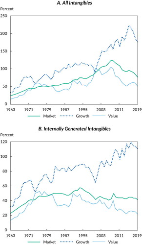
Notes: Panel A displays the ratio of all intangibles (capitalized R&D and 30% of SG&A plus acquired intangibles) to the tangible part of the book value of equity (the book value of equity minus acquired intangibles). Panel B displays the ratio of internally generated intangibles (capitalized R&D and 30% of SG&A) to the book value of equity.

Sources: Research Affiliates, LLC, using data from CRSP/Compustat; Peters and Taylor (2017).

Figure 2. Traditional B/P-Based HML vs. iHML Performance: US Market, July 1963–June 2020

Sources: Research Affiliates, LLC, using data from CRSP/Compustat.

Figure 3. The Return to Value from Three Elements

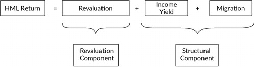
Table 3. Attribution of Value Factor Returns

Size	Valuation	Total Return (%)	Revaluation Premium (pps)	Structural Premium (pps)	Income Yield (pps)	Migration (pps)
A. Return decomposition, July 1963–June 2007
Small	Value – growth	8.4	0.1	8.3	–17.7	26.0
Big	Value – growth	3.8	0.3	3.5	–8.8	12.4
Average	HML	6.1	0.2	5.9	–13.2	19.2
B. Return decomposition, July 2007–June 2020
Small	Value – growth	–4.8	–4.9	0.2	–23.1	23.3
Big	Value – growth	–7.5	–9.6	2.0	–8.8	10.8
Average	HML	–6.1	–7.2	1.1	–15.9	17.0
C. Full-span return decomposition, July 1963–June 2020
Small	Value – growth	5.4	–1.1	6.5	–18.9	25.4
Big	Value – growth	1.2	–2.0	3.2	–8.8	12.0
Average	HML	3.3	–1.5	4.8	–13.9	18.7

Note: Log returns used in the attribution (see Appendix C).

Sources: Research Affiliates, LLC, using data from CRSP/Compustat.

Figure 4. HML Value Factor Performance and Relative Valuations: US Market, July 1963–June 2020

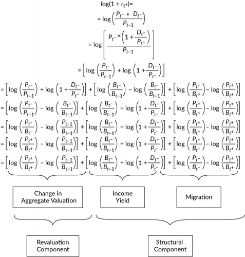
Notes: We computed the relative valuations each month by constructing a monthly rebalanced version of HML. The signal is the book value of equity from a fiscal year that ended at least six months earlier divided by the market value of equity lagged by six months. This signal matches the signal of the annually rebalanced HML: When HML was rebalanced at the end of June in year t, the book value of equity is from the fiscal year that ended in year t – 1 and the market value is from December of year t – 1. Our monthly version of HML matches the standard HML’s valuations at the rebalancing points while still tracing out valuations at a monthly frequency. Moreover, because most US companies have December fiscal year-ends, the value factor (HML) becomes predictably cheaper at the June rebalancing date. This rebalancing effect then dissipates over the following year. We removed the resulting seasonalities from valuations by subtracting the calendar month–specific (e.g., February) mean valuation and adding back the unconditional mean valuation. An alternative method for constructing a timely measure of value (and valuations) is the “HML devil,” which divides the lagged book value of equity by the current price (Asness and Frazzini 2013). The $r^{HML}$ is HML return, and $\Delta p{b}_t$ is the change in the logarithm of the price-to-book ratio.

Sources: Research Affiliates, LLC, using data from CRSP/Compustat.

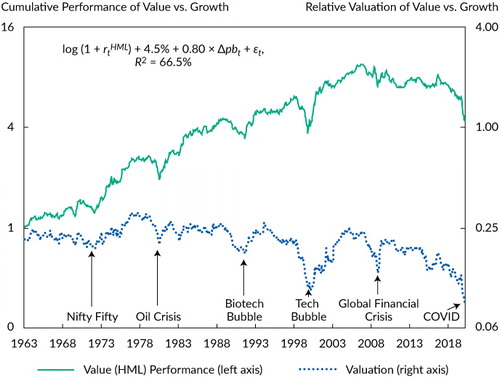
Table 4. Performance of Alternative Value Definitions: US Stocks

	July 1963–December 2006		January 2007–June 2020		July 1963–June 2020		Historical Percentile Rank		Raw Percentile Rank
Value Definition	Average	t-Stat.	Average	t-Stat.	Average	t-Stat.	June 2007	June 2020	June 2007	June 2020
HML (book to price)	5.6%	3.86	–5.4%	–2.00	3.0%	2.34	32%	100%	32%	100%
HML, small cap	7.5	4.33	–4.5	–1.69	4.6	3.14	60	100	63	100
HML, large cap	3.8	2.47	–6.2	–1.92	1.4	1.02	15	100	14	100
Value to neutral	2.4	3.40	–1.9	–1.06	1.3	1.98	54	98	52	98
Neutral to growth	3.3	2.73	–3.5	–2.38	1.7	1.71	14	100	14	100
iHML, ibook to price	6.7	5.17	–3.2	–1.27	4.3	3.73	5	100	3	100
E/P	5.2	3.08	–2.2	–0.93	3.5	2.46	39	88	37	91
S/P	5.8	4.01	–1.0	–0.51	4.2	3.46	25	98	25	98
Composite	4.9	2.87	–3.6	–1.34	2.9	1.98	44	95	43	95

Notes: In the value-to-neutral and neutral-to-growth definitions, neutral refers to the middle 40% of stocks by B/P. Recall that value comprises the 30% of stocks with the highest B/Ps and growth comprises the 30% of stocks with the lowest B/Ps. For the portfolios defined by intangibles-adjusted iHML, by the E/P, and by the S/P, we followed the HML convention: groups of 30% value, 40% neutral, and 30% growth. Each of the large-cap and small-cap universes were equally weighted by the respective large-cap or small-cap results for each of the value, growth, and neutral portfolios. We averaged earnings, sales, or dividends over the previous five years so that the portfolio definitions would be insensitive to cyclical peaks and troughs, following Arnott, Hsu, and Moore (2005). For the rightmost columns of percentile ranks, we measured the valuation percentiles in June 2007 and June 2020 by using the same ratio used to form the portfolios.

Sources: Research Affiliates, LLC, using data from CRSP/Compustat.

Figure 5. Historical Distribution of Relative HML Valuations: US Market, July 1963–June 2020

Notes: We estimated the theoretical distribution of valuations using kernel density estimation. We took the realized distribution of valuations from Figure 5 and used the Epanechnikov (parabolic) kernel with optimal bandwidth. This method can be considered to fit a smooth “density” over the historical histogram of valuations; it fills the gaps and makes educated guesses about the distribution outside the highest and lowest historical valuations. We have also placed the July 2007 and June 2020 relative valuations in this distribution plot.

Sources: Research Affiliates, LLC, using data from CRSP/Compustat.

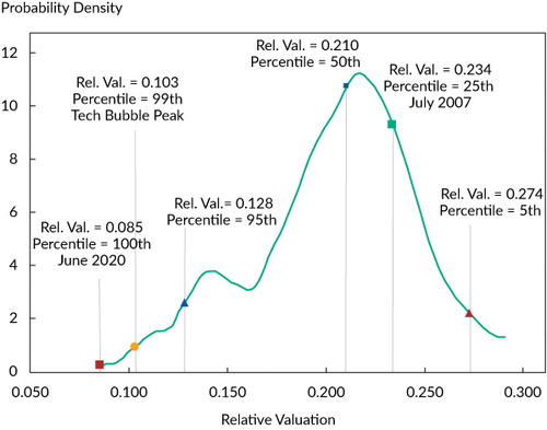
Table 5. Scenario Analysis: Forward-Looking Expected Return, Conditional on Revaluation

Directional Change	Scenario End Point	Relative Valuation	Log Relative Valuation Z-Score	Historical Percentile Rank	Return
Expanding relative valuations	Negative 6-σ deviation	0.061	–6.00	Beyond 100th	–21.8%
	Negative 5-σ deviation	0.075	–5.00	Beyond 100th	–5.3
	Zero premium	0.081	–4.68	Beyond 100th	0.0
No change	Stay at 100th percentile	0.085	–4.40	100th	4.5
Contracting relative valuations	Move to 95th percentile	0.128	–2.43	95th	37.1
	Move to 90th percentile	0.143	–1.90	90th	45.8
	Move to 75th percentile	0.181	–0.75	75th	64.8
	Move to 50th percentile	0.211	–0.02	50th	76.8
	Halfway mean reversion	0.134	–2.20	93th	40.8
Starting levels		0.085	–4.40	100th

Notes: For projections, we used a regression-based model that captures the relationship between year-over-year changes in relative valuations and contemporaneous returns. The model accounts for the potential cross-correlation between terms and was calibrated over the full sample of July 1963–June 2020. Shown are the regression results in Figure 3. Implied returns were trivially computed from this linear model once we knew the starting and ending points in the relative valuations. Similarly, we used the model to compute the level of changes in relative valuations required to generate a zero HML return in the first row of the table. We computed the halfway mean-reversion point by using the regression of the B/P-relative HML valuation against the year-earlier valuation.

Sources: Research Affiliates, LLC, using data from CRSP/Compustat.

Figure A1. Histogram of Largest Drawdowns for HML Value Factor Based on 1 Million Simulations

Note: Bootstrap simulations are drawn from US HML returns for July 1963–December 2006.

Sources: Research Affiliates, LLC, using CRSP/Compustat data.

Table B1. HML vs. iHML Spanning Tests: US Market, July 1963–June 2020 (t-statistics in parentheses)

	Dependent Variable: HML				Dependent Variable: iHML
	(1)	(2)	(3)		(4)	(5)	(6)
Alpha, annual	3.04*	3.97**	–0.19		4.34**	4.57**	1.34**
	(2.34)	(3.12)	(–0.36)		(3.73)	(3.90)	(2.64)
Market		–0.14**	–0.07**			–0.04	0.04**
		(–6.11)	(–6.73)			(–1.63)	(3.57)
Size			–0.21**				0.20**
			(–13.99)				(13.82)
Momentum			–0.02				–0.02
			(–1.56)				(–1.82)
Value (HML)							0.81**
							(53.74)
Value (iHML)			0.99**
			(56.26)
N	684	684	684		684	684	684
Adjusted R^2		5.0%	84.4%			0.2%	82.4%

Notes: Column numbers identify the individual models in the spanning tests. In columns 1–3, traditional HML was regressed on the market, size, and momentum factors (following Carhart 1997) as well as on iHML. Standard errors are clustered at the company level. Significance is measured under the assumption of a single hypothesis test.

* Significant at the 5% level.

** Significant at the 1% level.

Sources: Research Affiliates, LLC, using data from CRSP/Compustat.

Figure C1. The Return to Value from Three Elements: Detailed Examination