The COS method for option valuation under the SABR dynamics

Figures & data

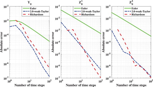
Figure 1. SABR example.

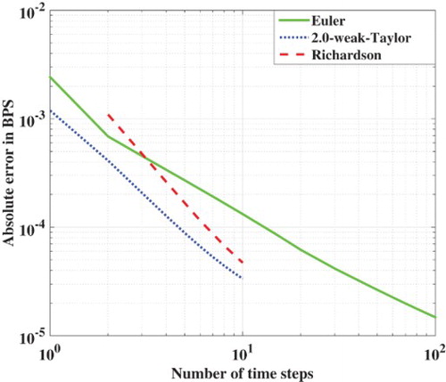
Table 1. Number of time steps and CPU time needed to obtain an absolute error of 1 or 0.5 basis points in the Black implied volatility for the Euler (with and without Richardson extrapolation) and 2.0-weak-Taylor schemes.

	M	CPU (s)	Absolute error in BPS
Euler	28	65.41	$<1$
2.0-weak-Taylor	5	143.56	$<1$
Richardson	8	24.62	$<1$
Euler	56	134.85	$<0.5$
2.0-weak-Taylor	7	235.42	$<0.5$
Richardson	10	33.94	$<0.5$

Figure 2. The Heston model with different correlations: (a) the Euler–Maruyama scheme and (b) Richardson extrapolation on the Euler results.

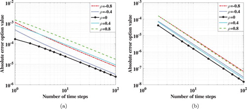
Figure 3. Heston Bermudan put with 5 early-exercise dates.

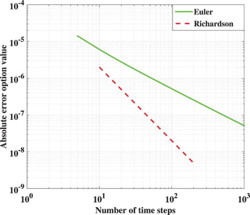
Figure 4. Geometric basket call option with the Euler scheme.

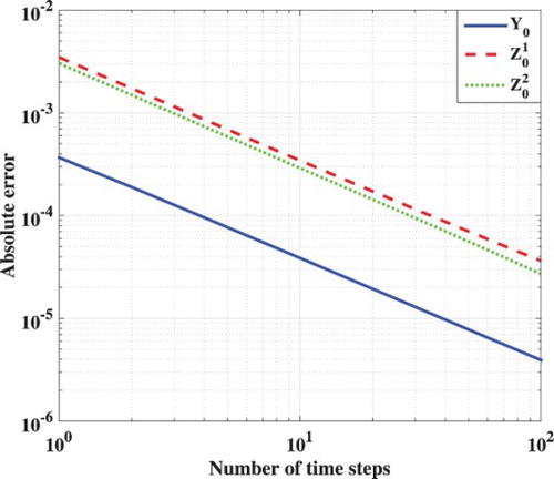
Figure 5. Spread option with the Euler scheme and CEV FSDEs (52(47) $\begin{array}{rl}{Z}_m^{1,\mathrm{\Delta }}\left(\mathbf{\text{x}}\right)& =\frac{1}{\mathrm{\Delta }t{\theta }_2}{\mathbb{E}}_m\left[Y_{m+1}^{\mathrm{\Delta }}\right({\mathbf{\text{X}}}_{m+1}^{\mathrm{\Delta }}\left)\mathrm{\Delta }{W}_{m+1}^1\right]-\frac{1-{\theta }_2}{{\theta }_2}{\mathbb{E}}_m\left[Z_{m+1}^{1,\mathrm{\Delta }}\right({\mathbf{\text{X}}}_{m+1}^{\mathrm{\Delta }})+\rho Z_{m+1}^{2,\mathrm{\Delta }}({\mathbf{\text{X}}}_{m+1}^{\mathrm{\Delta }}\left)\right]\\ & +\frac{1-{\theta }_2}{{\theta }_2}{\mathbb{E}}_m\left[f\right(t_{m+1},{\mathbf{\Lambda }}_{m+1}^{\mathrm{\Delta }}\left({\mathbf{\text{X}}}_{m+1}^{\mathrm{\Delta }}\right)\left)\mathrm{\Delta }{W}_{m+1}^1\right]-\rho Z_m^{2,\mathrm{\Delta }}\left(\mathbf{\text{x}}\right),\end{array}$(47) ).

Figure 6. SABR example.

Table 2. Number of time steps and CPU time needed to obtain a certain accuracy in option price for the Euler (with and without Richardson extrapolation) and 2.0-weak-Taylor schemes.

	M	CPU (s)	Absolute error $Y_0$
Euler	12	84.95	$<3\mathrm{e}-4$
2.0-weak-Taylor	3	203.54	$<3\mathrm{e}-4$
Richardson	6	53.89	$<3\mathrm{e}-4$
Euler	36	258.43	$<1\mathrm{e}-4$
2.0-weak-Taylor	6	504.92	$<1\mathrm{e}-4$
Richardson	8	82.09	$<1\mathrm{e}-4$