Drift-preserving numerical integrators for stochastic Poisson systems

Figures & data

Figure 1. Linear stochastic oscillator: numerical trace formulas for $\mathbb{E}[H(p(t),q(t))]$ on the interval $[0,5]$ (left) and $[0,100]$ (right). Comparison of the Euler–Maruyama scheme (EM), the stochastic trigonometric method (STM), the drift-preserving scheme (DP), the backward Euler–Maruyama scheme (BEM), and the exact solution.

Figure 2. Linear stochastic oscillator: mean-square convergence rates for the backward Euler–Maruyama scheme (BEM), the Euler–Maruyama scheme (EM), the drift-preserving scheme (DP), and the stochastic trigonometric method (STM). Reference lines of slopes 1, resp. 1/2.

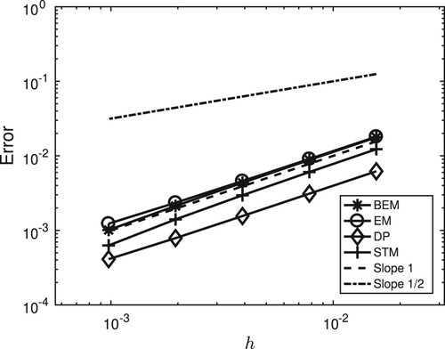
Figure 3. Linear stochastic oscillator: weak convergence rates for the backward Euler–Maruyama scheme (BEM), the Euler–Maruyama scheme (EM), the drift-preserving scheme (DP), and the stochastic trigonometric method (STM). Reference lines of slopes 1, resp. 2. (a) Errors in the first moments $\mathbb{E}[q(t)]$ (left) and $\mathbb{E}[p(t)]$ (right), (b) Errors in the second moments $\mathbb{E}[q(t{)}^2]$ (left) and $\mathbb{E}[p(t{)}^2]$ (right).

Figure 4. Linear stochastic oscillator: numerical trace formulas for $\mathbb{E}[H(p(t),q(t))]$ on the interval $[0,100]$. Comparison of the drift-preserving scheme (DP), the splitting methods with, respectively, the symplectic Euler method (SYMP), the Störmer-Verlet method (ST), the explicit Euler method (splitEULER), the Heun method (splitHEUN), and the exact solution.

Figure 5. Stochastic mathematical pendulum: numerical trace formulas for $\mathbb{E}[H(p(t),q(t))]$ on the interval $[0,100]$. Comparison of the drift-preserving scheme (DP), the splitting methods with, respectively, the symplectic Euler method (SYMP), the Störmer-Verlet method (ST), the explicit Euler method (splitEULER), and the exact solution.

Figure 6. Stochastic rigid body problem: numerical trace formulas for the energy $\mathbb{E}[H(X(t))]$ (left) and for the Casimir $\mathbb{E}[C(X(t))]$ (right) for the drift-preserving scheme (DP), the Euler–Maruyama scheme (EM), the backward Euler–Maruyama scheme (BEM), and the exact solution.

Figure 7. Stochastic rigid body problem: mean-square convergence rates for the backward Euler–Maruyama scheme (BEM), the drift-preserving scheme (DP), and the Euler–Maruyama scheme (EM). Reference lines of slopes 1, resp. 1/2.

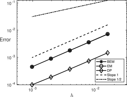
Figure 8. Stochastic rigid body problem: weak convergence rates in the first moment $\mathbb{E}[X_1(t_n)]$ (left) and second moment $\mathbb{E}[X_1(t_n{)}^2]$ (right) for the drift-preserving scheme (DP), the Euler–Maruyama scheme (EM), and the backward Euler–Maruyama scheme (BEM). Reference lines of slopes 1, resp. 2.

Figure 9. Stochastic rigid body problem with two-dimensional noise: numerical trace formulas for the energy $\mathbb{E}[H(X(t))]$ (left) and for the Casimir $\mathbb{E}[C(X(t))]$ (right) for the Casimir $\mathbb{E}[C(X(t))]$ (right) for the drift-preserving scheme (DP), the Euler–Maruyama scheme (EM), the backward Euler–Maruyama scheme (BEM), and the exact solution.