Figures & data
Figure 1. Illustration of the heavy top, where CM is the centre of mass of the body, O is the fixed point, is the gravitational acceleration vector, and
follow the notation introduced in Section 3.4.1.
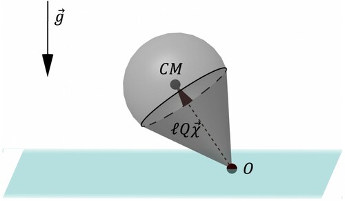
Figure 2. Symplectic Lie group integrators integration on the time interval . Left: 3D plot of
. Centre: components of
. The left and centre plots are computed with the same step-size. Right: verification of the order of the methods.
![Figure 2. Symplectic Lie group integrators integration on the time interval [0,1]. Left: 3D plot of MℓQ−1Γ0. Centre: components of QX. The left and centre plots are computed with the same step-size. Right: verification of the order of the methods.](/cms/asset/d4c820e0-eb02-4618-b144-27140c38c6ab/gcom_a_1966772_f0002_oc.jpg)
Figure 3. Symplectic Lie group integrators, long time integration, h = 0.01, 6000 steps.. Top: energy error, bottom 3D plot of .
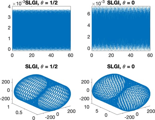
Figure 4. Threefold pendulum at a fixed time instant, with fixed point placed at the origin.
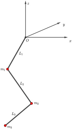
Figure 5. Convergence rate of the implemented Lie group integrators, based on global error considering as a reference solution the one of ODE45, with strict tolerance.
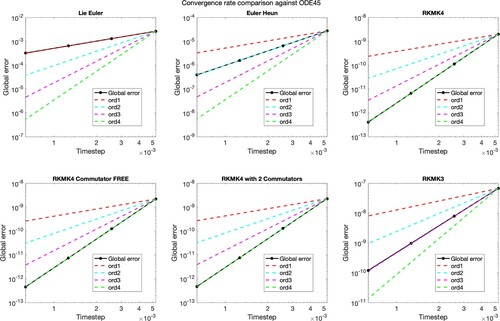
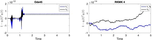
Figure 6. Visualization of the quantity , i = 1, 2, for time
. These plots focus on the preservation of the geometry of
.
![Figure 6. Visualization of the quantity 1−qi(t)Tqi(t), i = 1, 2, for time t∈[0,5]. These plots focus on the preservation of the geometry of S2.](/cms/asset/b92e8e84-8725-409c-b3fb-8c43b419e967/gcom_a_1966772_f0006_oc.jpg)
Figure 7. Visualization of the inner product , i = 1, 2, for
. These plots focus on the preservation of the geometry of
.
![Figure 7. Visualization of the inner product qi(t)Tωi(t), i = 1, 2, for t∈[0,5]. These plots focus on the preservation of the geometry of Tqi(t)S2.](/cms/asset/80b2a8ed-b80e-4733-a940-b1ac7f0badb7/gcom_a_1966772_f0007_oc.jpg)
Figure 8. Comparison of accuracy at final time (on the left) and step adaptation for the case N = 20 (on the right), with all pendulums of length .
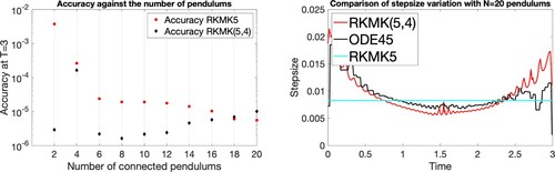
Figure 9. In these plots, we represent the six components of the solution describing the dynamics of the first mass (on the left) and of the second mass (on the right), for the case N = 2. We compare the behaviour of the solution obtained with constant stepsize RKMK5, the variable stepsize RKMK(5,4) and ODE45. (a) (b)
.
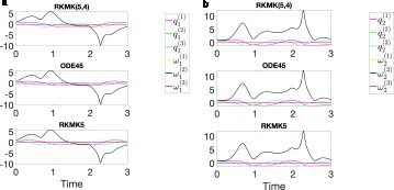
Figure 10. Comparison of accuracy at final time (on the left) and step adaptation for the case N = 20 (on the right), with all pendulums of length .
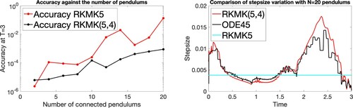
Figure 11. On the left, we compare the adaptation of the stepsize of RKMK(5,4) with the one of ODE45 and with the constant stepsize of RKMK5. In the centre, we plot the second component of the angular velocities , i = 1, 2, and we zoom in the last time interval
to see that the variable stepsize version of the method better reproduces the reference solution. On the right, we visualize the speed of variation of second component of the angular velocities. (a) Step adaptation, (b) Zoom at final times, (c) Values of
.
![Figure 11. On the left, we compare the adaptation of the stepsize of RKMK(5,4) with the one of ODE45 and with the constant stepsize of RKMK5. In the centre, we plot the second component of the angular velocities ωi(2), i = 1, 2, and we zoom in the last time interval t∈[2.1,3] to see that the variable stepsize version of the method better reproduces the reference solution. On the right, we visualize the speed of variation of second component of the angular velocities. (a) Step adaptation, (b) Zoom at final times, (c) Values of ω˙i(2)(t).](/cms/asset/173d8eef-e8b1-4a4f-9bb4-4b9c3b8650ca/gcom_a_1966772_f0011_oc.jpg)
Figure 12. Two quadrotors connected to the mass point via massless links of lengths
.
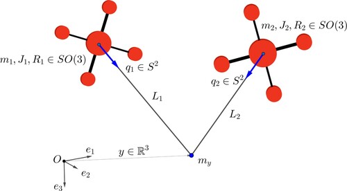
Figure 13. Convergence rate of the numerical schemes compared with ODE45.
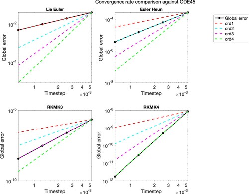
Figure 14. Snapshots at .
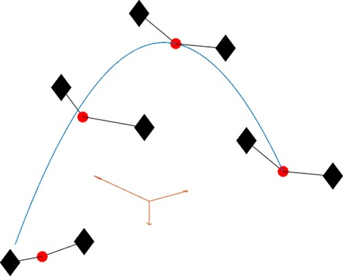
Figure 15. Components of the load position (in blue) and the desired trajectory (in red) as a function time.
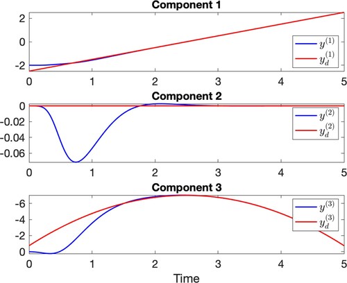
Figure 16. Deviation of the load position from the target trajectory.
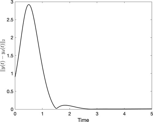
Figure 17. Direction error of the links.
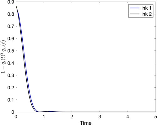
Figure 18. Preservation of the norms of .