Estimating stresses driving tissue flows using a stokes inverse problem

Figures & data

Figure 1. Particle Image Velocimetry (PIV) of cell flow velocity fields in epiblast of chicken embryo during primitive streak formation Figure Credit: C.J. Weijer Lab. White arrows show direction of tissue flow. The white scale bar is 300 $\mu$m in length and $4\mu \mathrm{m}{\min }^{-1}$ in tissue velocity.

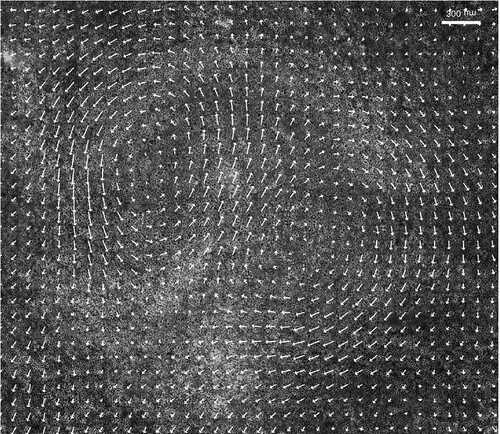
Figure 2. Velocity data and the mesh. (a) Experimental velocity field at stage HH2 of development. Velocity vectors are shown on a $28\times 20$ grid. The red scale bar is 0.5 millimeter in length. (b) Finite element mesh based on the velocity data.

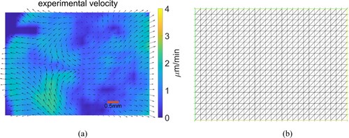
Figure 3. Comparing results. The red scale bar is 0.5 millimeter in length. (c) Experimental velocity at time $t_I$. (d) Experimental velocity at time $t_{II}$. (e) Numerical velocity at time $t_I$. (f) Numerical velocity at time $t_{II}$. (g) Numerical stress at time $t_I$. (h) Numerical stress at time $t_{II}$.

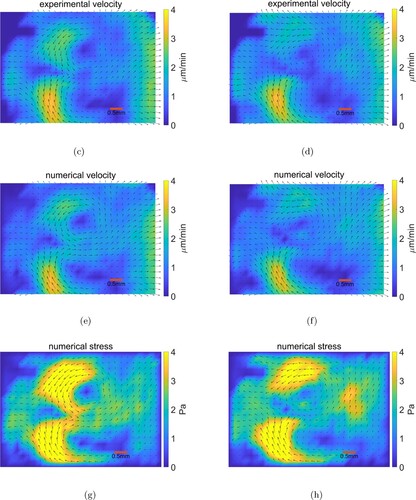
Figure 4. Comparing results. The red scale bar is 0.5 millimeter in length. (i) Experimental velocity at time $t_{III}$. (j) Experimental velocity at time $t_{IV}$ (k) Numerical velocity at time $t_{III}$ (l) Numerical velocity at time $t_{IV}$. (m) Numerical stress at time $t_{III}$ (n) Numerical stress at time $t_{IV}$.

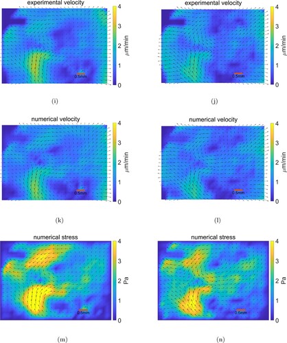
Table 1. The relative velocity error regarding to different time intervals.

Time interval	$t_I$	$t_{II}$	$t_{III}$	$t_{IV}$
Relative velocity error	$11.25\mathrm{\%}$	$9.30\mathrm{\%}$	$11.69\mathrm{\%}$	$11.89\mathrm{\%}$

Figure 5. Minimum value of $J_{h,\mathrm{\Omega }}(\mathbf{U},\mathbf{f})$ during the optimization process. (o) at $t_I$ (p) at $t_{II}$ (q) at $t_{III}$ (r) at $t_{IV}$.

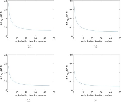
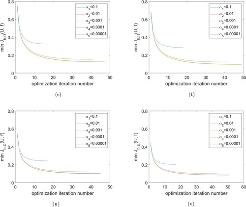
Table 2. Relationship between α and optimization iteration number.

	Optimization iteration number
Time intervals	${\alpha }_1=0.1$	${\alpha }_2=0.01$	${\alpha }_3=0.001$	${\alpha }_4=0.0001$	${\alpha }_5=0.00001$
$t_I$	17	41	47	48	48
$t_{II}$	18	42	48	49	49
$t_{III}$	17	39	45	45	46
$t_{IV}$	17	43	50	51	51

Figure 6. Minimum value of $J_{h,\mathrm{\Omega }}(\mathbf{U},\mathbf{f})$ during the optimization process for different values of α. (s) at $t_I$ (t) at $t_{II}$ (u) at $t_{III}$ (v) at $t_{IV}$.