A gradient-based calibration method for the Heston model

Figures & data

Table 1. Five initial values sets for ${\kappa }_{\nu }^{\mathrm{init}}$ for the different percentages and the corresponding calibrated values for C0.

${\kappa }_{\nu }^{\mathrm{init}}$	T1	T2	T3	T4	T5	${\kappa }_{\nu }^{\mathrm{cal}}$	T1	T2	T3	T4	T5
10	4.60	5.15	4.50	4.70	4.50	10	4.60	5.15	4.51	4.70	4.50
25	4.75	4.60	5.25	5.90	4.45	25	4.75	4.60	5.24	5.88	4.45
50	4.10	3.25	3.55	2.90	7.00	50	4.11	3.26	3.55	2.94	6.95
75	5.70	7.30	7.00	7.50	6.60	75	5.69	7.29	6.85	7.40	6.60

Table 2. Five initial values sets for ${\mu }_{\nu }^{\mathrm{init}}$ for the different percentages and the corresponding calibrated values for C0.

${\mu }_{\nu }^{\mathrm{init}}$	T1	T2	T3	T4	T5	${\mu }_{\nu }^{\mathrm{cal}}$	T1	T2	T3	T4	T5
10	0.0679	0.0637	0.0735	0.0714	0.0714	10	0.0598	0.0727	0.0575	0.0632	0.0577
25	0.0721	0.0777	0.0616	0.0630	0.0868	25	0.0655	0.0610	0.0720	0.0836	0.0615
50	0.1001	0.0406	0.0840	0.0448	0.0434	50	0.0476	0.0148	0.0484	0.0136	0.0882
75	0.0742	0.0532	0.0448	0.0399	0.0490	75	0.0847	0.1069	0.1005	0.1064	0.0928

Table 3. Five initial values sets for ${\sigma }_{\nu }^{\mathrm{init}}$ for the different percentages and the corresponding calibrated values for C0.

${\sigma }_{\nu }^{\mathrm{init}}$	T1	T2	T3	T4	T5	${\sigma }_{\nu }^{\mathrm{cal}}$	T1	T2	T3	T4	T5
10	0.465	0.545	0.510	0.515	0.480	10	0.451	0.559	0.484	0.502	0.455
25	0.575	0.570	0.505	0.415	0.480	25	0.565	0.546	0.523	0.455	0.429
50	0.580	0.360	0.630	0.345	0.655	50	0.501	0.292	0.581	0.261	0.713
75	0.705	0.470	0.235	0.350	0.565	75	0.718	0.562	0.390	0.489	0.630

Table 4. Five initial values sets for ${\rho }^{\mathrm{init}}$ for the different percentages and the corresponding calibrated values for C0.

${\rho }^{\mathrm{init}}$	T1	T2	T3	T4	T5	${\rho }^{\mathrm{cal}}$	T1	T2	T3	T4	T5
10	−0.550	−0.485	−0.520	−0.520	−0.495	10	−0.483	−0.547	−0.404	−0.460	−0.384
25	−0.410	−0.490	−0.605	−0.585	−0.380	25	−0.370	−0.390	−0.690	−0.829	−0.159
50	−0.555	−0.465	−0.350	−0.685	−0.725	50	−0.258	−0.242	−0.207	−0.441	−0.847
75	−0.695	−0.205	−0.775	−0.655	−0.150	75	−0.743	−0.972	−0.990	−0.990	−0.437

Table 5. Relative reduction of the cost functional computed with 31(31) $r({\xi }_{\mathrm{init}})=100\cdot (1-\frac{J(\tilde{V},{\xi }_{\mathrm{opt}})}{J(\tilde{V},{\xi }_{\mathrm{init}})}).$(31) using the different test cases for ${\xi }_{\mathrm{init}}$ and ${\xi }_{\mathrm{cal}}$ in the constant calibration setting.

C0	T1	T2	T3	T4	T5
10	43.12	77.38	65.22	63.22	52.75
25	58.46	78.38	62.14	66.06	64.53
50	83.09	20.84	52.76	30.98	72.62
75	16.23	72.89	82.89	82.09	80.43

Table 6. Different cases for calibration setting.

	${\kappa }_{\nu }$	${\mu }_{\nu }$	${\sigma }_{\nu }$	ρ
C0	constant	constant	constant	constant
C1	time-dependent	constant	constant	constant
C2	constant	time-dependent	constant	constant
C3	constant	constant	time-dependent	constant
C4	constant	constant	constant	time-dependent
C5	time-dependent	time-dependent	time-dependent	time-dependent
C6	constant	time-dependent	time-dependent	time-dependent
C7	constant	time-dependent	constant	time-dependent

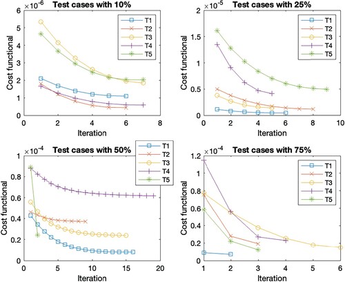
Figure 1. Cost functional evolution per iteration for the test cases within the constant parameter calibration.

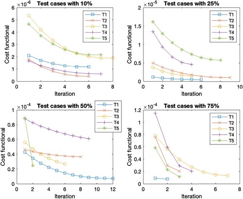
Table 7. Relative cost function reduction for the C1 calibration.

C1	T1	T2	T3	T4	T5
10	44.48	78.75	64.91	64.12	54.03
25	58.97	78.98	62.96	66.77	63.96
50	83.13	19.59	45.71	33.45	72.84
75	16.59	72.80	82.14	81.13	80.94

Table 8. Relative cost function reduction for the C2 calibration.

C2	T1	T2	T3	T4	T5
10	42.96	77.85	63.17	62.09	53.05
25	58.03	77.05	63.09	68.46	70.00
50	82.90	20.79	51.89	29.79	73.66
75	16.05	74.64	82.95	82.43	78.89

Table 9. Relative cost function reduction for the C3 calibration.

C3	T1	T2	T3	T4	T5
10	44.22	77.89	64.50	64.04	53.52
25	58.49	78.76	61.62	65.92	64.50
50	83.05	20.97	52.49	30.55	72.23
75	15.96	72.91	82.71	82.10	80.44

Table 10. Relative cost function reduction for the C4 calibration.

C4	T1	T2	T3	T4	T5
10	49.03	75.90	66.62	66.49	56.81
25	60.42	77.71	62.64	68.50	62.96
50	78.54	18.24	52.63	30.29	74.03
75	20.89	73.59	81.75	80.49	79.74

Table 11. Relative cost function reduction for the C5 calibration.

C5	T1	T2	T3	T4	T5
10	47.63	75.50	65.79	64.45	57.08
25	60.70	76.67	62.36	68.51	71.33
50	82.32	20.89	58.63	31.72	72.96
75	20.79	73.10	78.14	77.71	78.76

Table 12. Relative cost function reduction for the C6 calibration.

C6	T1	T2	T3	T4	T5
10	47.91	76.08	65.50	64.77	56.43
25	60.27	76.39	63.37	70.16	68.91
50	80.94	19.19	57.15	29.38	73.71
75	20.84	74.74	81.70	80.74	79.10

Table 13. Relative cost function reduction for the C7 calibration.

C7	T1	T2	T3	T4	T5
10	47.79	75.66	65.50	64.66	56.48
25	60.21	76.37	62.80	69.43	69.29
50	81.08	19.35	57.16	30.05	73.02
75	20.62	74.55	80.59	80.09	78.89

Table 14. Number of iterations for the different case scenarios for Tests 1, 3, and 5 within the $50\mathrm{\%}$ percentage difference in the initial parameter set.

Test cases	C0	C1	C2	C3	C4	C5	C6	C7
T1	12	12	13	12	12	17	16	16
T3	6	6	5	6	6	17	15	15
T4	9	9	19	9	9	19	19	19

Note: The bold cases illustrate the scenarios where ${\mu }_{\nu }$ is considered time dependent.

Table 15. Absolute difference between the largest and smallest relative cost functional reduction.

Difference	T1	T2	T3	T4	T5
10	5.91	2.39	2.12	3.27	4.33
25	2.67	2.61	1.75	4.24	8.37
50	4.59	2.73	12.92	4.07	1.41
75	4.93	1.94	4.81	4.29	2.85

Table 16. Average cost functional reduction in percentage for the different cases over the 20 test cases, as well as a list for the corresponding relative cost functional reduction as well as the figures of the cost functional evolution.

Case Setup	C0	C1	C2	C3	C4	C5	C6	C7
$r_a({\xi }_{\mathrm{init}})$	61.30	61.31	61.49	61.34	61.86	62.25	62.36	66.12
Table	5	7	8	9	10	11	12	13
Figure	1	2	3	4	5	6	7	8

Figure 2. Cost functional evolution per iteration for the different test set in the case scenario C1.

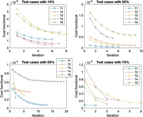
Figure 3. Cost functional evolution per iteration for the different test set in the case scenario C2.

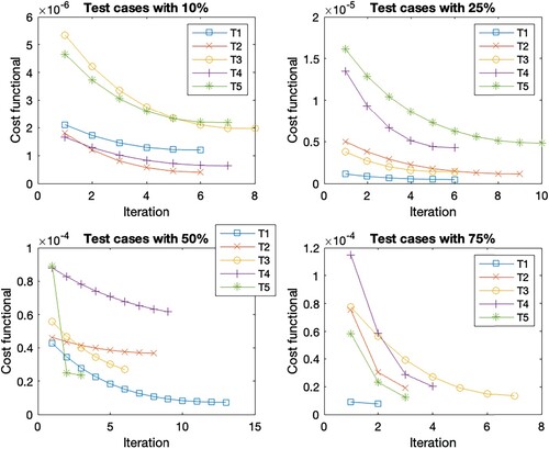
Figure 4. Cost functional evolution per iteration for the different test set in the case scenario C3.

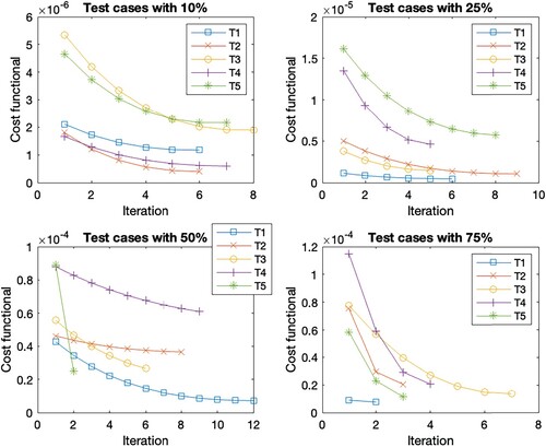
Figure 5. Cost functional evolution per iteration for the different test set in the case scenario C4.

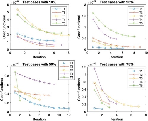
Figure 6. Cost functional evolution per iteration for the different test set in the case scenario C5.

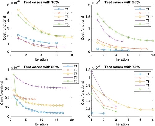
Figure 7. Cost functional evolution per iteration for the different test set in the case scenario C6.

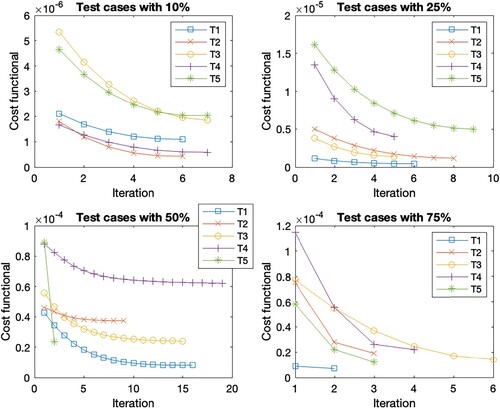
Figure 8. Cost functional evolution per iteration for the different test set in the case scenario C7.