Stable inversion of LPTV systems with application in position-dependent and non-equidistantly sampled systems

Figures & data

Figure 1. LPTV behaviour occurs in many mechatronic applications.

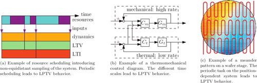
Figure 2. For nonminimum-phase system H, stable inversion yields bounded signal u such that y = r.

Figure 3. Input shift ${\mathcal{D}}_{-\rho }$ renders $\bar{H}$ bi-proper such that $\bar{H}$ is invertible. The shift is compensated through time-shifting output ${\bar{u}}_k$ of $\bar{F}={\bar{H}}^{-1}$ as $u_k={\mathcal{D}}_{-\rho }{\bar{u}}_k$. The results are exact on an infinite horizon.

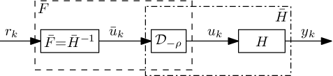
Figure 4. Stable inversion procedure for LPTV systems.

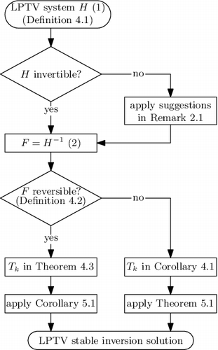
Figure 5. Time line of the non-equidistant sampling sequence. Control for the equidistant sampling sequence with period h = h ₀ + h ₁ is conservative since not all control points are exploited. To improve performance, control for the non-equidistant sampling sequence h ₀, h ₁ is pursued.

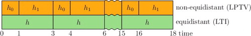
Figure 6. Stable inversion generates bounded u, whereas direct inversion generates unbounded u. The performance of stable inversion is limited due to finite preview. The performance of the equidistant sampled LTI system is low due to an inexact inverse.

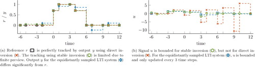
Figure 7. Additional preview improves the performance of stable inversion compared to Figure 6.

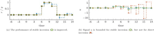
Figure 8. Application of stable inversion in ILC enables high-performance tracking with a nonexact model.

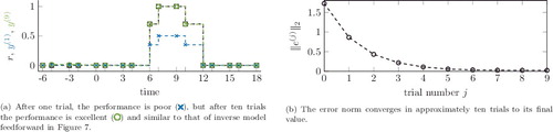
Figure 9. Top view of wafer stage. The interferometer is fixed on the metrology frame and measures distance $\widehat{x}$ to the wafer stage which has degrees of freedom x, y, φ. If φ ≠ 0, position y effects measurement $\widehat{x}$.

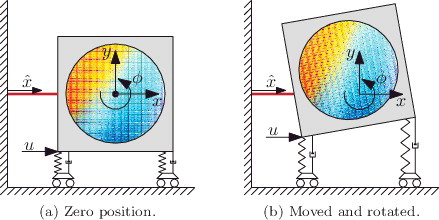
Table 1. Parameter values of the wafer stage system.

Parameter	Symbol	Value	Unit
Mass	m	50	kg
Inertia	I	2.08	kg m^2
Spring constant	c	10^6	N/m
Damping constant	d	2500	N s/m
Length	l	0.5	m

Figure 10. Part of meander pattern constructed by ${\widehat{x}}^d,y$ in Figure 11(a).

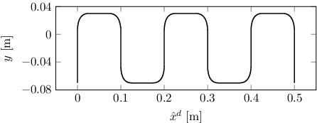
Figure 11. Prescribed position y introduces position-dependence resulting in an LPTV system that is unstable. With stable inversion, a bounded solution u resulting in perfect tracking is obtained.

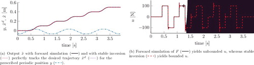
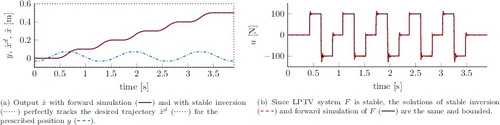
Figure 12. Prescribed position y introduces position-dependence resulting in an LPTV system that is stable. The stable inversion solution reduces to that of forward simulation and yields perfect tracking.