Huygens' clocks: ‘sympathy’ and resonance

Figures & data

Figure 1. Experimental setups with two metronomes placed in row configuration on a platform that is solely moving in one of the elementary directions: (a) horizontal displacement; (b) vertical displacement: the cables are suspended by springs and guided through the holes in metal strips.

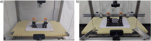
Figure 2. Experimental results, pendulum angles ${\theta }_1$: black and ${\theta }_2$: gray (top). (a) Horizontal system, in-phase synchronisation. (b) Vertical system, in-phase synchronisation. (c) Vertical system, anti-phase synchronisation.

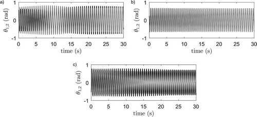
Figure 3. Experimental results with stiffer setups, pendulum angles ${\theta }_1$: black and ${\theta }_2$: gray (top). (a) Horizontal system in-phase synchronisation. (b) Horizontal system, anti-phase synchronisation. (c) Vertical system, quarter-phase synchronisation.

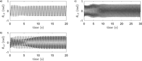
Table 1. Properties of the Nikko Lupina 311 metronome, experimentally found by the least square method, Hoogeboom et al. (2016).

Property	Value
Mass of pendulum	$m_p=18.5\mathrm{g}$
Mass of pendulum bob	$m_b=8.6\mathrm{g}$
Length of pendulum	$l_p=0.0245\mathrm{m}$
Length of pendulum bob	$l_b=0.027\mathrm{m}$
Damping constant	$d=0.0024\mathrm{Nmms}/\mathrm{rad}$
Gravitational acceleration	$g=9.81\mathrm{m}/{\mathrm{s}}^2$
Driving torque of escapement mechanism	$\mu =0.0451\mathrm{Nmm}$
Starting angle of escapement mechanism	${\theta }_s=-0.1920\mathrm{rad}$
Ending angle of escapement mechanism	${\theta }_e=0.2793\mathrm{rad}$
Accuracy constant	$\epsilon =0.05$ –
Natural frequency	$f_{mtr}=1.733\mathrm{Hz}$

Figure 4. Schematic representations of the experimental setups presented in Figure 1. Two metronomes (blue) coupled by a platform (gray) which motion is constricted by a linear spring-damper system. (a) Platform displaces horizontally (b) Platform displaces vertically.

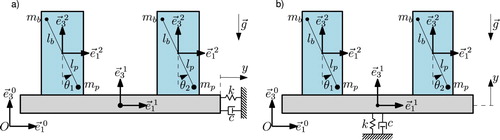
Table 2. Properties of the coupling platform (Pl), experimentally found by the least square method, Hoogeboom et al. (2016).

Property	Horizontal 1	Horizontal 2	Vertical 1	Vertical 2
Pl. mass, kg	M=0.3778	M=0.3778	M=0.433	M=0.433
Pl. stiffness, N/m	k=14.75	k=47.09	k=117.3	k=247.2
Pl. damping, Ns/m	c=0.0185	c=0.3868	c=0.0271	c=0.0592
Pl. eigenfreq., Hz	$f_{plt}=0.930$	$f_{plt}=1.661$	$f_{plt}=2.468$	$f_{plt}=3.584$

Figure 5. Numerical integration results of system (3(3a) $\begin{array}{rl}& M_t\ddot{y}+c\dot{y}+ky=-pf({\theta }_i,\dot{{\theta }_i},\ddot{{\theta }_i}),\end{array}$(3a) ), pendulum angles ${\theta }_1$: black and ${\theta }_2$: gray. (a) Horizontal system, in-phase synchronisation. (b) Vertical system, in-phase synchronisation. (c) Vertical system, anti-phase synchronisation. Compare this with Figure 2.

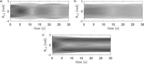
Figure 6. Bifurcation diagrams computed with Auto for systems (7(7a) $\begin{array}{rl}& {\tilde{y}}^{″}+2\zeta \frac{\mathrm{\Omega }}{\omega }{\tilde{y}}^{\prime }+\frac{{\mathrm{\Omega }}^2}{{\omega }^2}\tilde{y}=-\alpha f({\theta }_i,\dot{{\theta }_i},\ddot{{\theta }_i}),\end{array}$(7a) ). $\mathrm{\Delta }\phi =0$/$\frac{1}{2}\pi$/π denote in/quarter/anti-phase synchronisation and solid/dashed lines denote stable/unstable solutions. (a) Horizontal system, $f_{plt}=1.733\mathrm{Hz}$ and $f_{mtr}$ is bifurcation parameter. (b) Vertical system, $f_{plt}=1.733\mathrm{Hz}$ and $f_{mtr}$ is bifurcation parameter. (c) Horizontal system, $f_{mtr}=1.733\mathrm{Hz}$ and $f_{plt}$ is bifurcation parameter. (d) Vertical system, $f_{mtr}=1.733\mathrm{Hz}$ and $f_{plt}$ is bifurcation parameter.

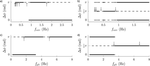
Figure 7. Numerical integration results of system (7(7a) $\begin{array}{rl}& {\tilde{y}}^{″}+2\zeta \frac{\mathrm{\Omega }}{\omega }{\tilde{y}}^{\prime }+\frac{{\mathrm{\Omega }}^2}{{\omega }^2}\tilde{y}=-\alpha f({\theta }_i,\dot{{\theta }_i},\ddot{{\theta }_i}),\end{array}$(7a) ) with $f_{mtr}=1.73\mathrm{Hz}$, pendulum angles ${\theta }_1$: black and ${\theta }_2$: gray. (a) Horizontal system, $f_{plt}=1.73\mathrm{Hz}$. (b) Vertical system, $f_{plt}=3.38\mathrm{Hz}$.

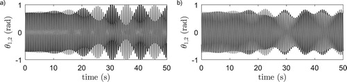
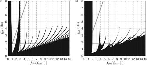
Figure 8. (a) Stability of the anti-phase solution of the horizontal system, White/black denote stable/unstable anti-phase behaviour. Gray lines correspond to stable anti-phase behaviour according to the local stability analysis of Figure 6(a,c), see the vertical arrows therein. (b) Stability of the quarter-phase solution of the vertical system, White/black denote stable/unstable quarter-phase behaviour. Gray lines correspond to stable quarter-phase behaviour according to the local stability analysis of Figure 6(b,d), see the vertical arrows therein.

Hoogeboom, F., Pogromsky, A., & Nijmeijer, H. (2016). Huygens' inspired multi-pendulum setups: Experiments and stability analysis. Chaos: An Interdisciplinary Journal of Nonlinear Science, 26, 116304. doi: 10.1063/1.4965031

 PubMed Web of Science ®Google Scholar