
Figures & data
Figure 1. Flowchart of the RBFNN optimal control algorithm with model reduction and transfer learning for linear systems.
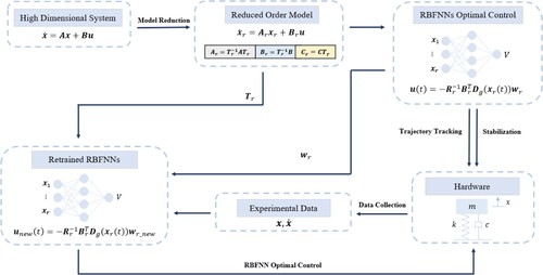
Figure 2. Quanser-Servo2 Inverted Pendulum system hardware setup (Quanser, Citation2022).
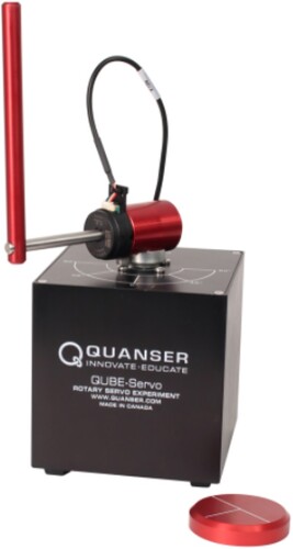
Table 1. Parameters of the rotary pendulum system.
Table 2. Summary of reduced order model matrices from model-based gramians and empirical gramians.
Table 3. Hankel singular values of the rotary pendulum.
Figure 3. Top: Relative output errors of the reduced order model by the balanced truncation and empirical balanced truncation. Below: The input signal.
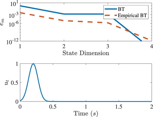
Figure 4. Tracking the square wave of the rotary army in simulations. In the legend, ‘LQR’ denotes the LQR control designed with the original model; ‘RBFNN’ denotes the RBFNN control designed with the model-based BT; ‘Empirical RBFNN’ denotes the RBFNN control designed with the empirical BT.
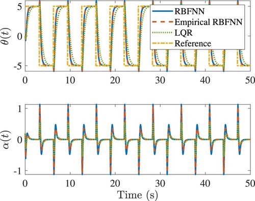
Figure 5. Comparisons of tracking response of the rotary army in simulations. In the legend, ‘RBFNN_Empirical’ denotes the RBFNN control designed with the empirical BT; ‘LQR_Empirical BT’ denotes the LQR control designed with the empirical BT; ‘LQR_Model-based BT’ denotes the LQR control designed with the model-based BT.
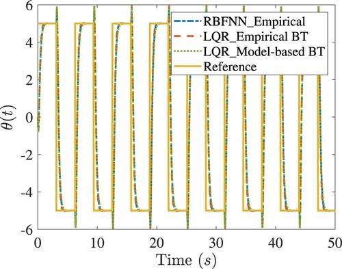
Figure 6. Comparisons of tracking response of the rotary army in simulations. Legends are the same as in Figure .
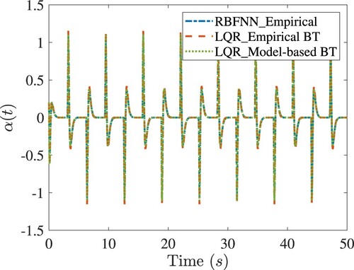
Figure 7. The closed-loop tracking responses of the rotary arm of Quanser-Servo2. Legends are the same as in Figure .
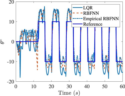
Figure 8. The closed-loop responses of the rotary arm under various controls for balancing the inverted pendulum of Quanser-Servo2. Top: Responses before retraining. Bottom: Responses after retraining. Legends are the same as in Figure .
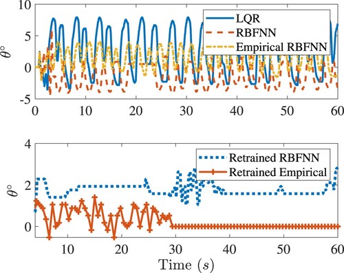
Figure 9. The closed-loop tracking response of the rotary arm of Quanser-Servo2. Legends are the same as in Figure .
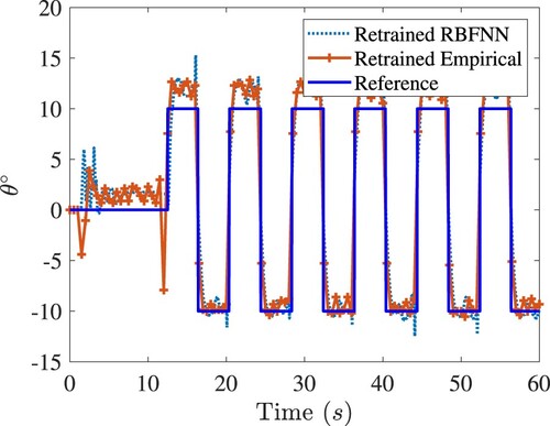
Figure 10. The closed-loop response of the pendulum in the rotary arm tracking control of Quanser-Servo2. Legends are the same as in Figure .
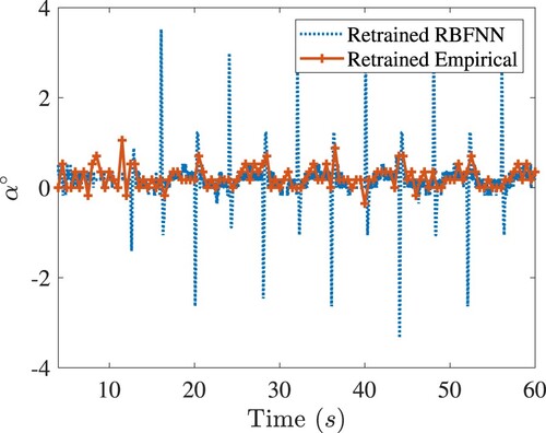
Table 4. Summary of control performance for LQR, RBFNN, empirical RBFNN, retrained RBFNN and retrained empirical RBFNN.
Figure 11. Robustness comparisons of all the controls under consideration. Top: The closed-loop angle response of the rotary arm in balancing control of Quanser-Servo2. Bottom: Disturbance
. Legends are the same as in Figure .
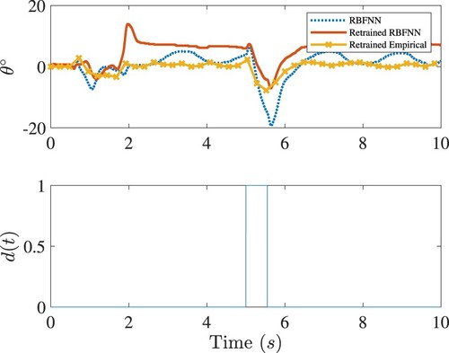
Figure 12. Disturbances to the second order nonlinear system.
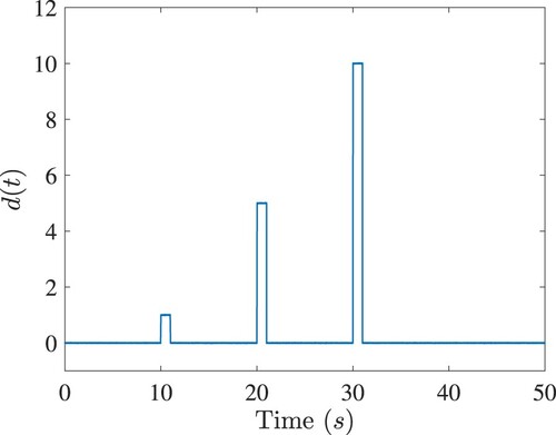
Figure 13. Performance comparison of RBFNN, Poly-NN control and LQR controls for the nonlinear system in Equation (Equation61(61)
(61) ). Top: The control
. Middle: The response
. Bottom: The response
.
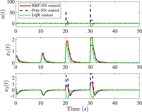
Figure 14. Comparison of spatial distribution of RBFNN and Poly-NN optimal controls u as a function of the state . Left: The control
plotted in the training region
. Right: The control
plotted beyond the training region into the larger region
.
![Figure 14. Comparison of spatial distribution of RBFNN and Poly-NN optimal controls u as a function of the state x. Left: The control u(x) plotted in the training region Xs1∈[−1,1]×[−1,1]. Right: The control u(x) plotted beyond the training region into the larger region Xs2∈[−2,2]×[−2,2].](/cms/asset/db99f4a6-3c95-4203-9bde-f43012e35e31/tcon_a_2328687_f0014_oc.jpg)
Figure 15. Robustness of the RBFNN and LQR controls with respect to the model uncertainty β. The vertical dash lines mark the critical value of β, beyond which the closed-loop system becomes unstable.
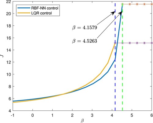
Figure A1. Comparison of RBFNNs and LQR control performances for the linear 2D system. Top: Control . Middle: Response
. Bottom: Response
. The initial condition of the system is
.
![Figure A1. Comparison of RBFNNs and LQR control performances for the linear 2D system. Top: Control u(t). Middle: Response x1(t). Bottom: Response x2(t). The initial condition of the system is x(0)=[1,1]T.](/cms/asset/2333d903-4fb1-4ce0-ac59-68b69e0a4db8/tcon_a_2328687_f0016_oc.jpg)