Modelling the evolution of human postmenopausal longevity using ordinary differential equations

Figures & data

Figure 1. Diagram of female-only model (1(1) $\begin{array}{rl}\frac{\mathrm{d}{F}_1}{\mathrm{d}t}& =\underset{\begin{array}{c}\mathrm{Offspring}\mathrm{produced}\mathrm{by}\\ \mathrm{young}\mathrm{and}\mathrm{old}{F}_1\\ \mathrm{females}\mathrm{with}\mathrm{no}\mathrm{mutation}\end{array}}{\underbrace{(1-\epsilon )(a+\mathrm{\gamma b})F_1}}-\underset{\mathrm{Death}}{\underbrace{\delta F_1}},\end{array}$(1) )–(2(2) $\begin{array}{rl}\frac{\mathrm{d}{F}_2}{\mathrm{d}t}& =\underset{\begin{array}{c}\mathrm{Offspring}\mathrm{produced}\mathrm{by}\\ \mathrm{young}\mathrm{and}\mathrm{old}{F}_1\\ \mathrm{females}\mathrm{with}\mathrm{mutation}\end{array}}{\underbrace{\epsilon (a+\mathrm{\gamma b})F_1}}+\underset{\begin{array}{c}\mathrm{Offspring}\mathrm{produced}\\ \mathrm{by}\mathrm{young}{F}_2\mathrm{females}\end{array}}{\underbrace{a{F}_2}}-\underset{\mathrm{Death}}{\underbrace{\delta F_2}},\end{array}$(2) ).

Table 1. Parameters and variables for (1(1) $\begin{array}{rl}\frac{\mathrm{d}{F}_1}{\mathrm{d}t}& =\underset{\begin{array}{c}\mathrm{Offspring}\mathrm{produced}\mathrm{by}\\ \mathrm{young}\mathrm{and}\mathrm{old}{F}_1\\ \mathrm{females}\mathrm{with}\mathrm{no}\mathrm{mutation}\end{array}}{\underbrace{(1-\epsilon )(a+\mathrm{\gamma b})F_1}}-\underset{\mathrm{Death}}{\underbrace{\delta F_1}},\end{array}$(1) )–(2(2) $\begin{array}{rl}\frac{\mathrm{d}{F}_2}{\mathrm{d}t}& =\underset{\begin{array}{c}\mathrm{Offspring}\mathrm{produced}\mathrm{by}\\ \mathrm{young}\mathrm{and}\mathrm{old}{F}_1\\ \mathrm{females}\mathrm{with}\mathrm{mutation}\end{array}}{\underbrace{\epsilon (a+\mathrm{\gamma b})F_1}}+\underset{\begin{array}{c}\mathrm{Offspring}\mathrm{produced}\\ \mathrm{by}\mathrm{young}{F}_2\mathrm{females}\end{array}}{\underbrace{a{F}_2}}-\underset{\mathrm{Death}}{\underbrace{\delta F_2}},\end{array}$(2) ).

Parameters	Description	Estimate
a	Reproductive contribution of young females in $F_1$ and $F_2$	$0.043{\mathrm{yr}}^{-1}$
b	Reproductive contribution of old females in $F_1$	$0.029{\mathrm{yr}}^{-1}$
γ	Probability an old female finds a mate	varies
δ	Death rate	$0.030{\mathrm{yr}}^{-1}$
ε	Probability of mutation	0.0001
Variables	Description
$F_1$	Female population with trait 1, lifelong fertility
$F_2$	Female population with trait 2, old-age infertility

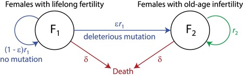
Figure 2. Survival curve from the Hadza lifetable of Blurton Jones et al. (2002, Table 3). We partition the population into three age classes: juvenile (age 0–15), young (age 15–45), and old (ages 45+).

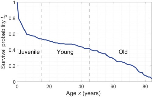
Figure 3. Growth curves dU/dt vs U for (4(4) $\frac{\mathrm{d}U}{\mathrm{d}t}=((1-\epsilon )(a+\mathrm{\gamma b})-a-\mathrm{\gamma bU})U.$(4) ). (a) When $0<1-\epsilon (1+a/b)$, the positive equilibrium is stable and U=0 is unstable. (b) When $0<1-\epsilon (1+a/b)$, the equilibrium at U=0 is stable and the negative equilibirum is unstable.

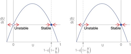
Figure 4. Bifurcation diagram of equilibrium points $U_{\mathrm{eq}}$ for the proportion of females with trait 1 (lifelong fertility) for various values of γ, the probability old, fertile females find mates. Equilibria cross at a transcritical bifurcation at $\gamma =(\epsilon /(1-\epsilon ))(a/b)$, where they swap stabilities.

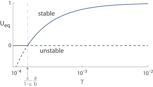
Figure 5. Phase plane for (11(11) $\begin{array}{rl}\frac{\mathrm{d}U}{\mathrm{d}t}& =(b(1-\epsilon -U)V-\mathrm{\epsilon a})U,\end{array}$(11) ) and (12(12) $\begin{array}{rl}\frac{\mathrm{d}V}{\mathrm{d}t}& =\mathrm{bUV}(1-V).\end{array}$(12) ). The population U is the proportion of females with lifelong fertility as opposed to old-age infertility, and V is the proportion of males who are unfussy and will mate with females of any age as opposed to fussy males who only mate young females. (Note that the figure is not drawn to scale to make certain features more prominent. In fact, it is generated by setting an artificially high mutation rate $\epsilon =0.05$ and taking other parameter values from Table 1.)

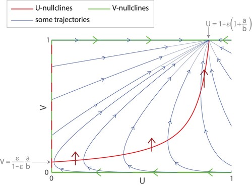
Figure 6. Trajectories for (11(11) $\begin{array}{rl}\frac{\mathrm{d}U}{\mathrm{d}t}& =(b(1-\epsilon -U)V-\mathrm{\epsilon a})U,\end{array}$(11) ) and (12(12) $\begin{array}{rl}\frac{\mathrm{d}V}{\mathrm{d}t}& =\mathrm{bUV}(1-V).\end{array}$(12) ) using parameters from Table 1, including $\epsilon =0.0001$. Nearly all trajectories approach the stable node at $(U,V)=(0.9998,1)$. The population U is the proportion of females with lifelong fertility as opposed to old-age infertility, and V is the proportion of males who are unfussy and will mate with females of any age as opposed to fussy males who only mate young females.

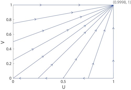
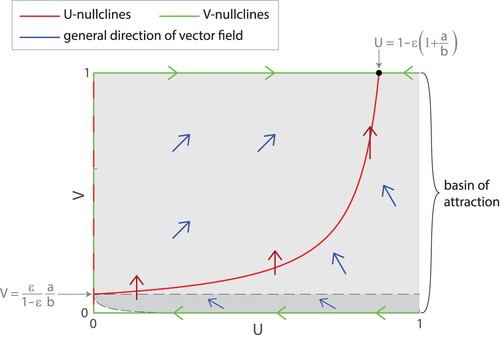
Figure 7. Basin of attraction for the stable node $(1-\epsilon (1+a/b),1)$. We can observe that all trajectories starting in the light grey region with U>0 and $V>(\epsilon /(1-\epsilon ))(a/b)$ have positive dV/dt and are repelled from the line of equilibria at U=0, so they are guaranteed to approach the stable node $(1-\epsilon (1+a/b),1)$. From numerical simulations, we find that the basin of attraction includes an additional region in dark grey below the dashed line $V=(\epsilon /(1-\epsilon ))(a/b)$. (Note that this figure is not drawn to the correct scale as in Figure 6. It is drawn to the scale of Figure 5.).

Blurton Jones, N. G., Hawkes, K., & O'Connell, J. F. (2002). Antiquity of postreproductive life: Are there modern impacts on hunter-gatherer postreproductive life spans? American Journal of Human Biology, 14(2), 184–205. https://doi.org/10.1002/ajhb.v14:2

 PubMed Web of Science ®Google Scholar