Cost modelling of onboard cobot-supported item sorting in a picking system

Figures & data

Table 1. Notations and example values.

			Example value(s)
Area	Notation	Description	Mode 1	Mode 2
Cost	$c_o$	Hourly cost (€/h) of an operator	[10; 20; 30; 40]	[10; 20; 30; 40]
	$c_e^j$	Yearly cost (€/year) of equipment in mode $j$	15,000	25,000
	$c_q^m$	Unitary cost (€/error) of correcting an error at picking area ($m=1$), at assembly ($m=2$), and at end of line inspection ($m=3$)	See Table 5	See Table 5
System	$n_d$	No. of orders to complete in a year	[10,000; 20,000; 30,000]	[10,000; 20,000; 30,000]
	$n_s$	No. of order lines per order	[5; 10; 15; 20]	[5; 10; 15; 20]
	$n_w$	No. of work days in a year	261	261
	$q_s$	No. of items per order line	[1; 2; 3; 4]	[1; 2; 3; 4]
	$t_h$	No. of hours in a work day	8	8
	$t_w$	No. of seconds in a work day	28,800	28,800
	${\mu }_s$	Order commonality	[0.15; 0.3; 0.5]	[0.1; 0.3; 0.5]
Process	$B$	Batch size	[2; 4; 8; 16]	[2; 4; 8; 16]
	$j$	Index for picking mode	1	2
	$k$	Index for error type	[1; 2; 3; 4; 5]	[1; 2; 3; 4; 5]
	$L$	Length (m) of a picking tour	[25; 50; 100; 200]	[25; 50; 100; 200]
	$n_s^{\mathrm{\prime }}$	No. of order lines on a batch pick list	–	–
	$q_s^{\mathrm{\prime }}$	No. of items per order line on a batch pick list	–	–
	$q_{tot}$	No. of items to pick on a picking tour with batch size $B$	–	–
	$t_{OL}^j$	Time (s) required to complete an order line on a batch pick list in mode $j$	–	–
	$t_{pick}$	Time (s) for the operator to pick a component	5	5
	$t_{set}$	Time (s) for setup between picking tours	30	30
	$t_{sort}^j$	Time (s) required to sort an item in mode $j$	4.5	8
	$v$	Travelling speed (m/s)	1	1
	$\delta$	Collaboration ratio	–	–
	$\varphi$	Collaboration factor	–	–
	${\rho }_{\epsilon }^k$	Probability of error type $k$	See Table 6	See Table 6
	${\pi }_p^j$	Probability of correcting an error at the picking area in mode $j$	0.95	0.99
	${\pi }_a$	Probability of correcting an error at the internal customer	0.7	0.7
	${\mu }_b$	Order commonality inverse	–	–
	${\delta }_l$	Average distance per order line	[1.25; 2.5; 5; 10; 20; 40]	[1.25; 2.5; 5; 10; 20; 40]
Model output	$\mathrm{\Delta }{C}_{tot}$	Relative cost difference between modes 1 and 2	–	–
	$C_O^j$	Yearly operator cost in mode $j$	–	–
	$C_E^j$	Yearly equipment cost in mode $j$	–	–
	$C_Q^j$	Yearly quality cost in mode $j$	–	–
	$C_{tot}^j$	Yearly total cost of mode $j$	–	–
	$p^j$	Productivity (order lines/year) in mode $j$	–	–
	$n_{op}^j$	No. of operators required in mode $j$	–	–

Figure 1. Overview of the manual sorting mode (top) and the cobot sorting mode (bottom).

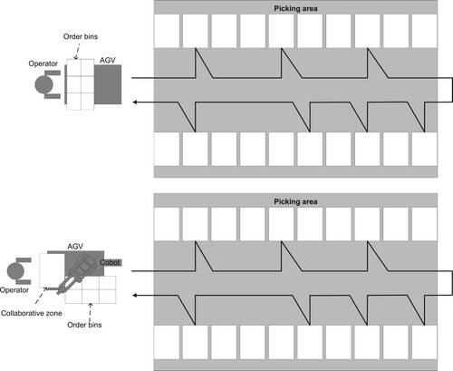
Table 2. Example of a pick list for one order.

Order line	Quantity	Order bin	SKU ID	Item no.	Item description
1	$q_1$	1	A01	123 456 789	Small bearing
2	$q_2$	1	A03	456 123 789	Medium bearing
3	$q_3$	1	A07	789 567 123	Grey plastic cap
$⋮$	$⋮$	$⋮$	…	…	…
$n_s$	$q_{n_s}$	1	…	…	…

Table 3. Example of a batch pick list for a setup with $B=8$, $q_s=1$.

Order line	Quantity	Order bin(s)	SKU ID	Item no.	Item description
1	4	1, 2, 5, 8	A01	123 456 789	Small bearing
2	3	3, 6, 7	A03	456 123 789	Medium bearing
3	8	1, 2, 3, 4, 5, 6, 7, 8	A07	789 567 123	Grey plastic cap
…	$⋮$	…	…	…	…
$n_s^{\mathrm{\prime }}$	$q_{n_s^{\mathrm{\prime }}}^{\mathrm{\prime }}$	…	…	…	…

Table 4. Equipment related costs associated with the two modes.

Manual sorting $\left(j=1\right)$	Cobot sorting $\left(j=2\right)$
AGV for transporting order bins and travelling in the warehouse (depreciation cost) Manual sorting support system on the AGV (depreciation cost of diodes, displays, wifi equipment/cables) Maintenance cost of sorting support system (covered in maintenance of shelf pick-by-light)	AGV for transporting order bins and travelling in the warehouse (depreciation cost) Cost of cobot (depreciation cost) Cost of cobot maintenance Licensing costs of cobot-control software

Table 5. Types and example values of error correction costs.

Correction type (m)	Description	Notation	Cost
1	Error is detected and corrected at picking area	$c_q^{m=1}$	0.05 €/error
2	Error is detected and corrected at assembly workstation	$c_q^{m=2}$	3.5 €/error
3	Error is corrected at end of line inspection	$c_q^{m=3}$	18.5 €/error

Table 6. Example values for error probabilities.

Error type	Description	${\rho }_{\epsilon }^k$
$k=1$	Missing item error	0.02
$k=2$	Wrong item error	0.02
$k=3$	Item unfit for use or damaged error	0.01
$k=4$	Incorrect number of items error	0.01
$k=5$	Items in wrong sequence or position error	0.04

Figure 2. Main cost components in €/year (logarithmic scale) of the two modes with respect to operator cost (left), equipment cost (middle), and quality cost (right). Boxes represent average cost and standard deviation. Bracketed lines represent maximum and minimum cost.

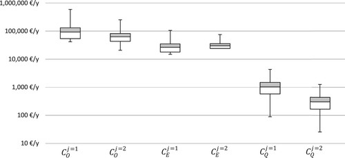
Figure 3. Main effect plot of $\mathrm{\Delta }{C}_{tot}$, showing effect size (vertical axis) and factor levels (horizontal axis) for the considered factors.

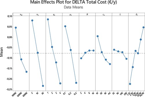
Figure 4. Interaction plot with respect to $\mathrm{\Delta }{C}_{tot}$, showing size of interaction effects (vertical axis) and the factor levels used for each parameter (horizontal axis).

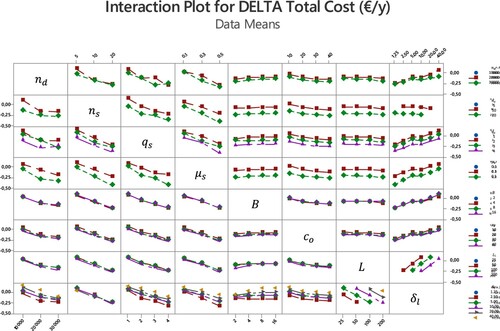
Figure 5. Relative cost difference between the manual sorting mode and the cobot sorting mode with respect to $n_d$ (vertical axis) and $q_s$ (horizontal axis) under different levels of ${\mu }_s$ and ${\delta }_l$. Grey areas indicate a more profitable manual sorting mode and white areas indicate a more profitable cobot sorting mode.

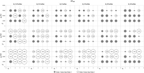
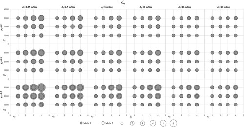
Figure 6. The average number of picking units required in mode 1 and 2 with respect to $n_d$ (vertical axis) and $q_s$ (horizontal axis) under different levels of ${\mu }_s$ and ${\delta }_l$. Grey circle without border indicate the average number of picking units required with mode 1, and hollow circle with border indicate the average number of picking units required with mode 2.