A novel self-training semi-supervised deep learning approach for machinery fault diagnosis

Figures & data

Figure 1. Overview of the framework of the proposed SSDL.

A labelled dataset is used to train a SSAE-Softmax model first, the model is then employed to predict the pseudo labels for the unlabelled samples based on the extracted features, and an enlarged training dataset by selecting some pseudo-labelled samples is finally generated to retrain the model.

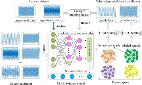
Figure 2. Structure of SAE and SSAE-Softmax neural network: (a) symmetrical structure neural network of SAE, where $x$ is the dimension of each sample, $g$ is the number of neurons in the hidden layer 1; and (b) structure of SSAE-Softmax classifier, where $d$ and $q$ are the number of neurons in the hidden layer 2 and hidden layer 3, respectively, $P(h=i|x)$ denotes the probability that $s$ is classified as operational state $i$ ($i=1,2,\dots ,y$).

Two subfigures, where the first one is the symmetrical structure neural network of SAE, and the second one is the structure of SSAE-Softmax classifier.

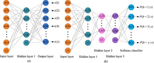
Figure 3. Flowchart of constructing SSDL model for machinery fault diagnosis.

Flowchart of constructing SSDL model for machinery fault diagnosis, which contains the sensor signal collection, sample generation and data division, semi-supervised deep feature learning, classifier training using deep features, SSDL model for machinery fault diagnosis, and application of the proposed model.

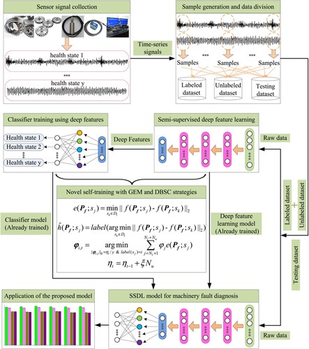
Table 1. Description of the four datasets for bearing fault diagnosis.

Dataset 1 (BD-1)			Dataset 2 (BD-2)			Dataset 3 (BD-3)			Dataset 4 (BD-4)
O	L	D	O	L	D	O	L	D	O	L	D
1	N	0	1	N	0	1	N	0	1	N	0
2	IR	7	2	IR	7	2	IR	7	2	IR	7
3	BA	7	3	IR	14	3	BA	7	3	BA	7
4	OR-3	7	4	IR	21	4	IR	14	4	OR-6	7
–	–	–	–	–	–	5	BA	14	5	IR	14
–	–	–	–	–	–	6	IR	21	6	BA	14
–	–	–	–	–	–	7	BA	21	7	OR-6	14
–	–	–	–	–	–	–	–	–	8	IR	21
–	–	–	–	–	–	–	–	–	9	BA	21
–	–	–	–	–	–	–	–	–	10	OR-6	21

Figure 4. Experimental data preparation for delta 3-D printer: (a) test-rig; (b) installed attitude sensor; (c) normal and fault state of a synchronous belt; and (d) normal and fault state of a joint bearing screw.

Four subfigures, where the first one is the test-rig of a delta 3-D printer, the second one is the attitude sensor, the third one is the normal and fault state of a synchronous belt, the last one is the normal and fault state of a joint bearing screw.

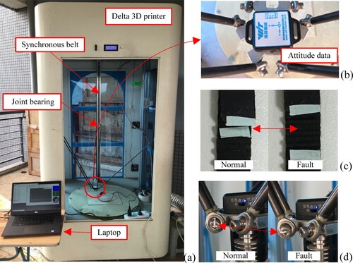
Table 2. Description of the four datasets for 3-D printer fault diagnosis.

Dataset 1 (PD-1)		Dataset 2 (PD-2)		Dataset 3 (PD-3)		Dataset 4 (PD-4)
O	State	O	State	O	State	O	State
1	N	1	N	1	N	1	N
2	JB-1	2	JB-1	2	JB-1	2	JB-1
3	JB-2	3	JB-2	3	JB-2	3	JB-2
4	JB-3	4	JB-3	4	JB-3	4	JB-3
–	–	5	JB-4	5	JB-4	5	JB-4
–	–	6	JB-5	6	SB-1	6	JB-5
–	–	–	–	7	SB-2	7	JB-6
–	–	–	–	8	SB-3	8	SB-1
–	–	–	–	–	–	9	SB-2
–	–	–	–	–	–	10	SB-3

Table 3. Diagnosis accuracies of SSDL under different combinations of network architecture and enlarging factor.

	$\xi$=1/3		$\xi$=1/5		$\xi$=1/10		$\xi$=1/15		$\xi$=1/30
Network architecture	avg	std	avg	std	avg	std	avg	std	avg	std
[100]	84.64	8.46	87.38	4.84	88.57	5.04	86.25	6.57	91.49	5.86
[200]	90.18	1.97	90.54	0.68	90.14	0.49	91.72	2.10	91.88	1.17
[300]	83.75	0.83	89.73	2.41	89.38	3.31	90.18	0.74	90.45	1.52
[400]	84.94	2.09	87.50	1.51	92.50	3.04	88.04	1.03	91.25	0.89
[500]	87.68	0.82	86.52	0.27	91.25	3.57	87.50	3.93	90.18	0.89
[600]	82.77	6.52	89.29	3.04	91.61	0.52	91.31	6.23	90.63	5.81
[100-100]	87.50	0.76	95.24	1.17	97.44	0.14	96.13	1.43	97.97	0.33
[200-200]	94.88	2.70	96.73	1.36	96.07	0.51	96.96	0.95	98.57	0.91
[300-300]	93.04	2.46	96.25	1.30	99.64	0.38	98.87	0.73	99.52	0.55
[400-400]	92.50	1.39	96.67	0.74	99.22	0.59	98.45	2.06	99.64	0.25
[500-500]	91.31	4.26	96.61	1.82	95.12	5.27	94.11	3.79	95.45	0.45
[600-600]	93.45	1.33	94.00	2.70	96.72	2.66	95.30	2.70	96.07	1.43
[50-50-50]	87.56	2.88	88.15	6.65	94.65	2.86	98.49	0.63	96.79	1.79
[100-100-100]	90.30	1.18	95.89	0.58	95.77	1.38	98.57	1.51	98.87	0.60
[150-150-150]	91.34	2.59	93.66	2.23	93.66	0.53	95.90	1.97	95.72	2.15
[200-200-200]	92.14	2.29	93.15	2.04	94.64	2.34	96.70	0.99	95.18	0.47
[250-250-250]	91.70	2.41	94.56	2.24	93.84	1.34	96.26	0.71	98.04	1.43
[300-300-300]	94.40	1.05	95.81	1.70	98.67	0.63	97.05	2.41	97.80	2.38

Table 4. Hyper-parameter settings for all the approaches on bearing datasets.

Approach	BD-1	BD-2	BD-3	BD-4
SSDL-SS	na = [500-500]; threshold = 0.95; iter = 10;	na = [200-200-200]; threshold = 0.95; iter = 5;	na = [200-200-200]; threshold = 0.98; iter = 10;	na = [300-300]; threshold = 0.88; iter = 10;
SSDL-SC	na = [300-300]; $\xi$=1/10;	na = [300-300]; $\xi$=1/30;	na = [200-200-200]; $\xi$=1/30;	na = [250-250-250]; $\xi$=1/30;
SSDL-ES	na = [400-400]; $\xi$=1/30;	na = [50-50-50]; $\xi$=1/15;	na = [50-50-50]; $\xi$=1/30;	na = [100-100-100]; $\xi$=1/30;
SSDL	na = [300-300]; $\xi$=1/10;	na = [50-50-50]; $\xi$=1/30;	na = [300-300]; $\xi$=1/30;	na = [300-300-300]; $\xi$=1/30;

Table 5. Hyper-parameter settings for all the approaches on 3-D printer datasets.

Approach	PD-1	PD-2	PD-3	PD-4
SSDL-SS	na = [100-100-100]; threshold= 0.98; iter = 5;	na = [100-100-100]; threshold= 0.95; iter = 10;	na = [300-300]; threshold = 0.95; iter = 10;	na = [400-400]; threshold = 0.95; iter = 10;
SSDL-SC	na = [150-100]; $\xi$=1/15;	na = [200-100-100]; $\xi$=1/15;	na = [400-300]; $\xi$=1/15;	na = [400-300]; $\xi$=1/30;
SSDL-ES	na = [200-100-100]; $\xi$=1/15;	na = [200-200-100]; $\xi$=1/15;	na = [300-300]; $\xi$=1/30;	na = [400-400]; $\xi$=1/15;
SSDL	na = [100-100-100]; $\xi$=1/30;	na = [100-100-100]; $\xi$=1/30;	na = [300-300]; $\xi$=1/15;	na = [400-400]; $\xi$=1/30;

Figure 5. The prediction accuracies obtained by all the algorithms on each testing dataset.

The prediction accuracies obtained by the SSDL-SS, SSDL-SC, SSDL-ES, and SSDL on datasets BD-1, BD-2, BD-3, BD-4, PD-1, PD-2, PD-3, and PD-4.

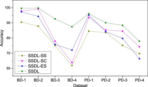
Figure 6. The iterative Accu and Accs values of the contrastive approaches on the BD-1: (a) SSDL-SS; (b) SSDL-SC; (c) SSDL-ES; and (d) SSDL.

Four subfigures are drawn to show the iterative Accu and Accs values of the SSDL-SS, SSDL-SC, SSDL-ES, and SSDL on dataset BD-1.

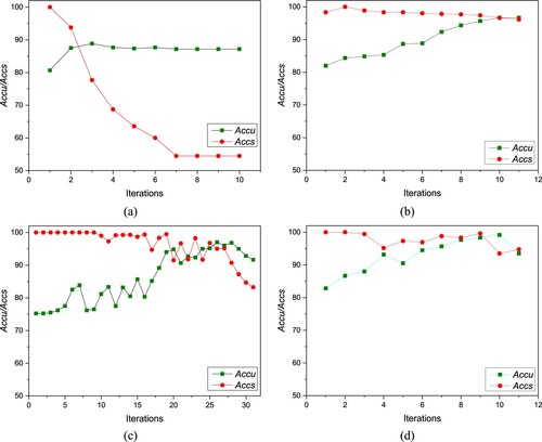
Figure 7. The iterative Accu and Accs values of the contrastive approaches on the BD-4: (a) SSDL-SS; (b) SSDL-SC; (c) SSDL-ES; and (d) SSDL.

Four subfigures are drawn to show the iterative Accu and Accs values of the SSDL-SS, SSDL-SC, SSDL-ES, and SSDL on dataset BD-4.

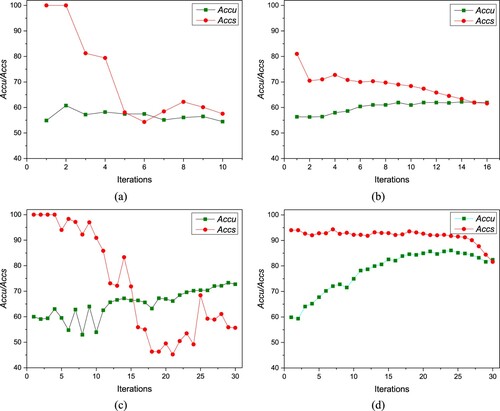
Figure 8. The prediction accuracies obtained by SSDL under different number of labelled samples on datasets PD-3 and PD-4.

The prediction accuracies obtained by SSDL on datasets PD-3 and PD-4 when the number of labelled samples is 10, 15, 20, 25, and 30.

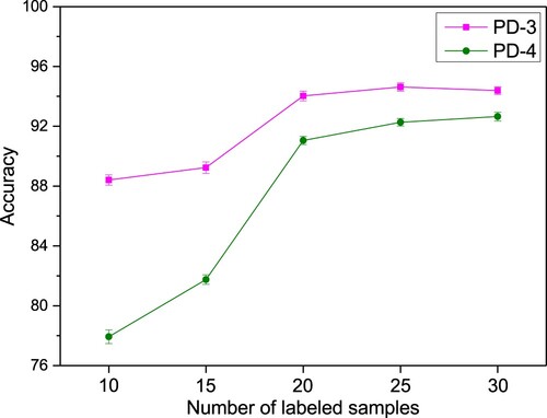
Table 6. Comprehensive comparison of diagnosis accuracy.

Dataset	mixmatch	MT	LTI	SSDL	BFS	BSU
BD-1	98.46 ± 0.13	98.29 ± 0.21	99.02 ± 0.18	99.64 ± 0.03	82.32 ± 0.27	100.00 ± 0.00
BD-2	98.41 ± 0.20	97.54 ± 0.19	98.76 ± 0.14	99.78 ± 0.02	84.47 ± 0.15	100.00 ± 0.00
BD-3	89.17 ± 0.36	87.28 ± 0.35	90.69 ± 0.32	92.65 ± 0.25	72.04 ± 0.31	97.02 ± 0.14
BD-4	83.85 ± 0.31	81.19 ± 0.41	84.12 ± 0.34	87.43 ± 0.21	59.43 ± 0.28	96.57 ± 0.18
PD-1	93.89 ± 0.26	93.26 ± 0.28	95.04 ± 0.23	95.98 ± 0.14	82.99 ± 0.17	98.35 ± 0.09
PD-2	87.18 ± 0.30	85.36 ± 0.33	88.21 ± 0.21	90.12 ± 0.23	81.22 ± 0.26	96.58 ± 0.13
PD-3	82.45 ± 0.27	79.43 ± 0.36	84.67 ± 0.29	88.41 ± 0.18	72.24 ± 0.36	95.83 ± 0.18
PD-4	73.76 ± 0.29	72.89 ± 0.33	75.03 ± 0.24	77.93 ± 0.21	61.85 ± 0.34	93.68 ± 0.21