The effects of supply variability on the performance of assembly systems

Figures & data

Table 1. Summary of previous work on the effect of variability of feeding stations on the performance of assembly systems

		Effect of …
Reference	Problem setting	Work transfer	Feeding stations’ Var (or CV)	Variability transfer
(W. J. Hopp and Simon 1989; W. J. Hopp and Simon 1993; Baker, Powell, and Pyke 1993; Powell and Pyke 1998)	2 symmetric feeding stations + 1 assembly station	WT to feeding stations increases TH
(Sabuncuoglu, Erel, and Kok 2002)	N symmetric feeding stations + 1 assembly station	WT to feeding stations (increase of feeding station mean processing times) increases TH and reduces IDV when CV = 1		VT to feeding stations (increase of feeding station processing time variance) increases TH and reduces IDV
(Krishnamurthy, Suri, and Vernon 2004)	2 asymmetric feeding stations, no assembly station, semi-open queueing network		Increasing Var reduces TH
(Boeck and Vandaele 2008; Boeck and Vandaele 2011)	2 asymmetric feeding stations, no assembly station		Increasing Var increases synchronisation time
(Manitz and Tempelmeier 2012)	General assembly line with multiple converging stations		Increasing Var increases IDV
(N. Chen et al. 2022)	Two converging, parallel assembly lines into a single, serial line		Increasing CV increases CV of assembly cycle time. No effect of Var on mean assembly cycle time

Table 2. Factors and their levels.

Factor	Levels	Values
Type of assembly system	2	YXY (X being AS) and XYY (X being FS1)
WT (work transfer)	19	MeanA (YXY) or Mean1 (XYY) from 0.1 to 1.9 minutes in 0.1 increments
Variability factor changed	2	Var or SCV
SumVar or SumSCV	3	1, 3 and 8
VT (variability transfer)	6	Var1 = 0 and Var2 = VarA = (1/2)SumVar  Var1 = 0, Var2 = (2/3)SumVar, VarA = (1/3)SumVar Var1 = (1/6)SumVar and Var2 = VarA = (5/12)SumVar Var1 = Var2 = VarA = (1/3) SumVar Var1 = Var2 = (5/12)SumVar and VarA = (1/6)SumVar Var1 = Var2 = (1/2)SumVar and VarA = 0 Equivalently for SCVi values

Figure 1. Illustration of the two types of assembly systems considered in the study.

Flow diagrams showing the characteristics of (a) symmetrical assembly systems and (b) asymmetrical assembly systems.

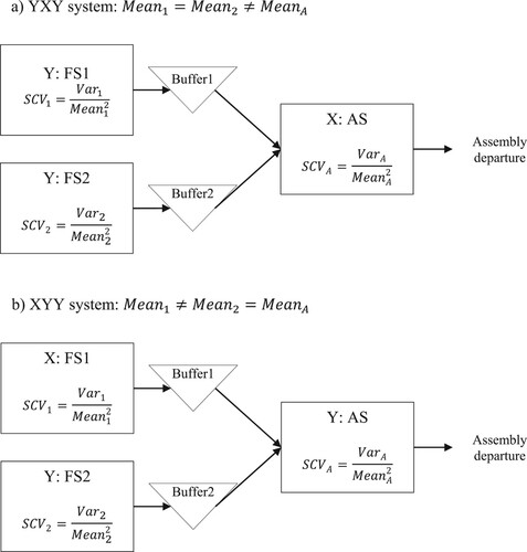
Table 3. List of abbreviations used throughout the manuscript.

Abbreviation	Variable
TH	Throughput rate of the assembly system
WT	Work transfer
IDV	Variance of inter-departure times
CV	Coefficient of variation
VT	Variability transfer
IDCV	Coefficient of variation of inter-departure times
Var	Variance
AS	Assembly station
FS1	Feeding station 1
FS2	Feeding station 2
SCV	Squared coefficient of variation
SumVar	Sum of variances of the three stations in the system
SumSCV	Sum of squared coefficients of variation of the three stations in the system
IDSCV	Squared coefficient of variation of inter-departure times
TA	Time spent in the assembly station
nTA	Normalised time spent in the assembly station
nρ	Normalised percentage capacity utilisation of the assembly station

Figure 2. TH for different levels of WT and VT, (a) SumVar = 1, (b) SumVar = 8, YXY systems.

Plots comparing the throughput rate of experiments with varying values of work and variability transfer for symmetrical scenarios with (a) SumVar = 1 and (b) SumVar = 8.

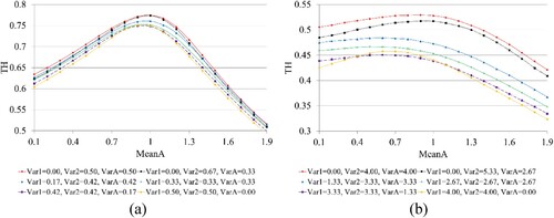
Figure 3. Normalised percentage capacity utilisation levels of the assembly station by different feeding variability and SumVar values, YXY systems.

Plot showing the effect of feeding variability on the normalised percentage capacity utilisation levels of the assembly station for different SumVar values in symmetrical systems.

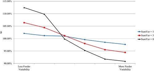
Figure 4. IDSCV for different values of WT and VT, (a) SumSCV = 1, (b) SumSCV = 8, YXY systems.

Plots comparing the squared coefficient of variation of inter-departure times for experiments with varying values of work and variability transfer for symmetrical scenarios with (a) SumVar=1 and (b) SumVar=8.

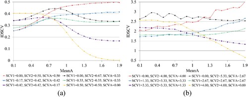
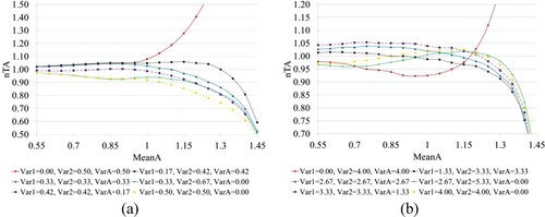
Figure 5. nTA for different values of WT and VT, (a) SumVar = 1, (b) SumVar = 8, YXY systems.

Plots comparing the normalised time spent in the assembly station for experiments with varying values of work and variability transfer for symmetrical scenarios with (a) SumVar=1 and (b) SumVar=8.

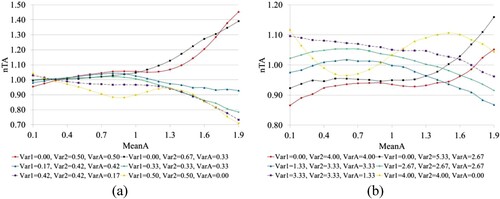
Figure 6. TH for different levels of WT and VT, (a) SumVar = 1, (b) SumVar = 8, XYY systems.

Plots comparing the throughput rate of experiments with varying values of work and variability transfer for asymmetrical scenarios with (a) SumVar=1 and (b) SumVar=8.

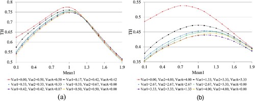
Figure 7. IDSCV for different values of WT and VT, (a) SumSCV = 1, (b) SumSCV = 8, XYY systems.

Plots comparing the squared coefficient of variation of inter-departure times for experiments with varying values of work and variability transfer for asymmetrical scenarios with (a) SumVar=1 and (b) SumVar=8.

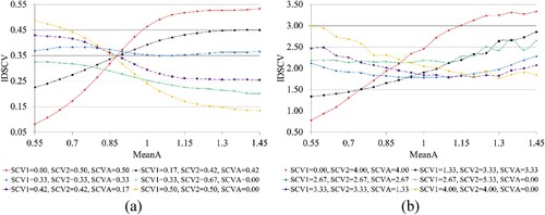
Figure 8. nTA for different values of WT and VT, (a) SumVar = 1, (b) SumVar = 8, XYY systems.

Plots comparing the normalised time spent in the assembly station for experiments with varying values of work and variability transfer for asymmetrical scenarios with (a) SumVar=1 and (b) SumVar=8.

Hopp, Wallace J, and John T Simon. 1989. “Bounds and Heuristics for Assembly-Like Queues.” Queueing Systems 4 (2): 137–155. doi:10.1007/BF01158549.

 Google Scholar

Hopp, Wallace J, and John T Simon. 1993. “Estimating Throughput in an Unbalanced Assembly-Like Flow System.” International Journal of Production Research 31 (4): 851–868. doi:10.1080/00207549308956762.

 Web of Science ®Google Scholar

Baker, Kenneth R, Stephen G Powell, and David F Pyke. 1993. “Optimal Allocation of Work in Assembly Systems.” Management Science 39 (1): 101–106. doi:10.1287/mnsc.39.1.101.

 Web of Science ®Google Scholar

Powell, Stephen G, and David F Pyke. 1998. “Buffering Unbalanced Assembly Systems.” IIE Transactions 30 (1): 55–65. doi:10.1080/07408179808966437.

 Web of Science ®Google Scholar

Sabuncuoglu, Ihsan, Erdal Erel, and A. Gurhan Kok. 2002. “Analysis of Assembly Systems for Interdeparture Time Variability and Throughput.” IIE Transactions 34 (1): 23–40. doi:10.1080/07408170208928847.

 Web of Science ®Google Scholar

Krishnamurthy, Ananth, Rajan Suri, and Mary Vernon. 2004. “Analysis of a Fork/Join Synchronization Station with Inputs from Coxian Servers in a Closed Queuing Network.” Annals of Operations Research 125 (1): 69–94. doi:10.1023/B:ANOR.0000011186.14865.19.

 Web of Science ®Google Scholar

Boeck, Liesje De, and Nico Vandaele. 2008. “Coordination and Synchronization of Material Flows in Supply Chains: An Analytical Approach.” International Journal of Production Economics 116 (2): 199–207. doi:10.1016/j.ijpe.2008.06.010.

 Web of Science ®Google Scholar

Boeck, Liesje De, and Nico Vandaele. 2011. “Analytical Analysis of a Generic Assembly System.” International Journal of Production Economics 131 (1): 107–114. doi:10.1016/j.ijpe.2010.04.036.

 Web of Science ®Google Scholar

Manitz, Michael, and Horst Tempelmeier. 2012. “The Variance of Inter-Departure Times of the Output of an Assembly Line with Finite Buffers, Converging Flow of Material, and General Service Times.” OR Spectrum 34 (1): 273–291. doi:10.1007/s00291-010-0216-1.

 Web of Science ®Google Scholar

Chen, Nan, Ningjian Huang, Robert Radwin, and Jingshan Li. 2022. “Analysis of Assembly-Time Performance (ATP) in Manufacturing Operations with Collaborative Robots: A Systems Approach.” International Journal of Production Research 60 (1): 277–296. doi:10.1080/00207543.2021.2000060.

 Web of Science ®Google Scholar

Data availability statement

The data that support the findings of this study are available from the corresponding author, RRS, upon reasonable request.