Intelligent machine fault diagnosis with effective denoising using EEMD-ICA- FuzzyEn and CNN

Figures & data

Figure 1. A calculation from the input to the output in the convolutional layer.

An computing example of the convolutional layer, the input feature mapping X is convolved with the convolution kernel. It can obtain the net input Z by adding a bias b in the convolution results. After a nonlinear activation function, the output feature mapping Y is obtained.

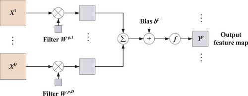
Figure 2. The overall framework of the proposed method.

The flowchart of this paper: firstly, simulating the different sensor noise levels, including slight noise, medium noise, strong noise, and extreme noise; secondly, the original signal and noisy signals will be denoised by a novel two-stage denoising method, named EEMD-ICA-FuzzyEn; finally, the denoised signals will be as the input data into the improved CNN model for intelligent fault diagnosis.

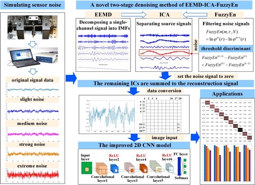
Figure 3. Test rig of rolling-element bearing.

Photograph of test rig of rolling-element bearing, it sequentially includes the electric motor, torque transducer & encoder, and dynamometer. And the accelerometers are installed on both the fan-end and the drive-end of the electric motor, which can measure the acceleration data of the test bearings.

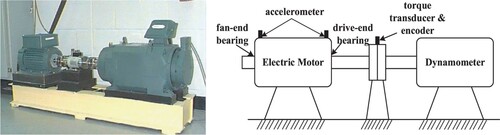
Table 1. The structure of the data sets.

Fault Diameter (in)	Fault Types	Number of training/ validation/testing samples	Class Label
0	normal bearing(NB)	500/300/200	C1
0.007” (slight fault)	inner race fault (IRF)	500/300/200	C2
	ball fault (BF)	500/300/200	C3
	outer race fault (ORF)	500/300/200	C4
0.014” (moderate fault)	inner race fault (IRF)	500/300/200	C5
	ball fault (BF)	500/300/200	C6
	outer race fault (ORF)	500/300/200	C7
0.021” (severe fault)	inner race fault (IRF)	500/300/200	C8
	ball fault (BF)	500/300/200	C9
	outer race fault (ORF)	500/300/200	C10

Figure 4. Different levels of Gaussian noise disturbance in normal bearing.

The amplitude of the original signal and four different noisy signals, increasing vibration amplitude as noise disturbance increases.

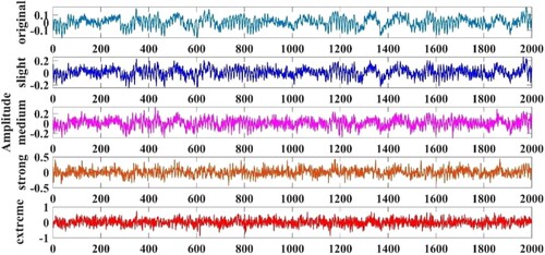
Figure 5. The decomposition results using EEMD of normal bearing.

The decomposed several intrinsic mode functions components by using the method of ensemble empirical mode decomposition (EEMD), containing high frequencies, low frequencies, and a residence of the signal.

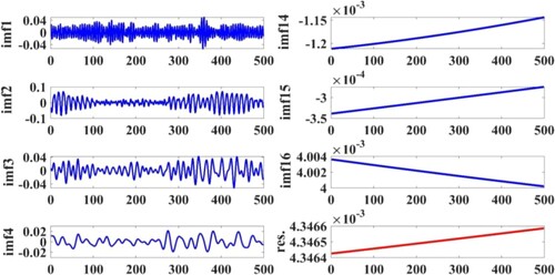
Figure 6. The separation results using Fast ICA-FuzzyEn under normal condition.

The independent components are separated from the multi-channel intrinsic mode functions by using the FastICA algorithm. And two independent components presented with the red line are filtered as the noise signals with fuzzy entropy values as the threshold criterion.

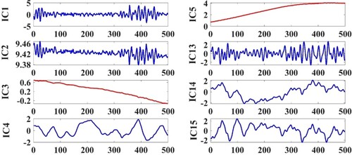
Figure 7. The original, noisy, and denoised signal of C3.

Choosing the rolling slight fault as an example, it presents the difference of amplitude among the original signal, added noise signal, and denoised signal.

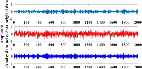
Figure 8. Evaluation denoising results among different noise levels.

The picture on the left is the correlation coefficient between the noisy signals and denoised signals under original data and different noise levels; the right graph is the root mean square error values between them. And the darker the colour, the larger the number.

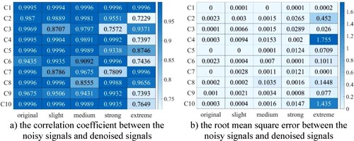
Table 2. Parameter settings of the EEMD-ICA-FuzzyEn and CNN model.

Method	Parameters	Value
EEMD	noise standard deviation (Nstd)	0.2
	number of realizations (Yang, Liu, and Zio)	50
	maximum number of sifting iterations allowed (MaxIter)	50
ICA	approach	Deflation
	nonlinearity approach	Power3
	stabilization	off
FuzzyEn	standard deviation (SD)	r = 0.2
	number of continuous variables	m = 2
	threshold discriminant	Satisfy
Improved CNN	convolution kernel 1	Weights 5*5*1*20; bias 1*1*20
	relu function 2	ReLU
	pooling layer 3	Maxpooling 2*2
	convolution kernel 4	Weights 5*5*20*40; bias 1*1*40
	relu function 5	ReLU
	convolution kernel 6	Weights 5*5*40*100; bias 1*1*100
	relu function1 7	ReLU
	batch_normalisation 8	Batch_normalisation
	full-connected layers 9	Weights 10*25600; bias 10*1
	softmax 10	Softmax

Figure 9. The repeated diagnosis results in denoised data with different noise levels.

The accuracy results in ten trials, with original data and different denoised data as input data to the improved CNN, outperform with high accuracy and slight influence by noise interference.

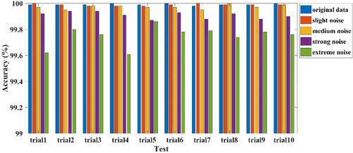
Figure 10. Confusion matrix with the original data and extreme noise as representatives.

The picture presents diagnosis performance for original data and extreme noise by the confusion matrix. And the highlighted diagonal values represent the correctly classified sample number of each state, and the other displaying red values belong to misclassified samples.

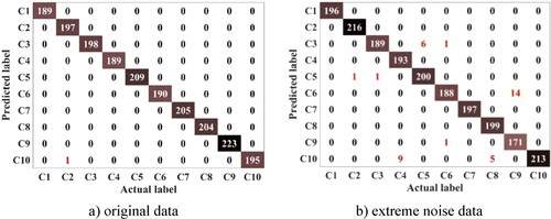
Table 3. Fault diagnosis performance comparison of noisy data and denoising data.

Noise level	Accuracy (%)	Recall (%)	Precision (%)	F1 score (%)
original	99.99 / 99.96	99.96 / 99.79	99.96 / 99.79	99.96 / 99.79
slight	99.99 / 99.89	99.94 / 99.46	99.95 / 99.46	99.95 / 99.46
medium	99.97 / 99.71	99.86 / 98.53	99.87 / 98.53	99.86 / 98.52
strong	99.91 / 99.14	99.55 / 95.75	99.55 / 95.83	99.55 / 95.73
extreme	99.75 / 96.91	98.77 / 84.58	98.75 / 85.87	98.75 / 84.18

Table 4. Comparison of diagnostic accuracy with other denoising methods.

Method	Original Data	Slight noise	Medium noise	Strong noise	Extreme noise
EEMD-FuEn-ICA	99.99	99.99	99.97	99.91	99.75
EMD-FuEn-ICA	99.99	99.95	99.82	99.72	99.08
EEMD	99.96	99.90	99.77	99.31	97.36

Table 5. Comparison of diagnostic accuracy with other DL approaches.

Method	Original Data	Slight noise	Medium noise	Strong noise	Extreme noise
The proposed method (denoised)	99.99	99.99	99.97	99.91	99.75
The proposed method (no denoising)	99.96	99.89	99.71	99.14	96.91
Ensemble TICNN (Zhang et al. 2018)	99.71	99.48	96.04	68.29	/
LDR-CNN (Ma et al. 2019)	100	99.82	99.45	98.88	97.36
Deep Transfer Learning(Li et al. 2019)	98.92	97.16	96.65	93.41	/
AAnNet(Jin et al. 2020)	99.83	99.66	99.83	98.97	59.31
MCNN-LSTM (Chen, Zhang, and Gao 2021)	98.46	88.19	81.41	77.27	/

Zhang, Wei, Chuanhao Li, Gaoliang Peng, Yuanhang Chen, and Zhujun Zhang. 2018. “A Deep Convolutional Neural Network with new Training Methods for Bearing Fault Diagnosis Under Noisy Environment and Different Working Load.” Mechanical Systems and Signal Processing 100:439–453.

 Web of Science ®Google Scholar

Ma, Shangjun, Wenkai Liu, Wei Cai, Zhaowei Shang, and Geng Liu. 2019. “Lightweight Deep Residual CNN for Fault Diagnosis of Rotating Machinery Based on Depthwise Separable Convolutions.” IEEE Access 7: 57023–57036.

 Web of Science ®Google Scholar

Li, Xiang, Wei Zhang, Qian Ding, and Xu Li. 2019. “Diagnosing Rotating Machines with Weakly Supervised Data Using Deep Transfer Learning.” IEEE Transactions on Industrial Informatics 16 (3): 1688–1697.

 Web of Science ®Google Scholar

Jin, Guoqiang, Tianyi Zhu, Muhammad Waqar Akram, Yi Jin, and Changan Zhu. 2020. “An Adaptive Anti-Noise Neural Network for Bearing Fault Diagnosis Under Noise and Varying Load Conditions.” IEEE Access 8: 74793–74807.

 Web of Science ®Google Scholar

Chen, Xiaohan, Beike Zhang, and Dong Gao. 2021. “Bearing Fault Diagnosis Base on Multi-Scale CNN and LSTM Model.” Journal of Intelligent Manufacturing 32 (4): 971–987.

 Web of Science ®Google Scholar

Data availability statement

The data that support the findings of this study are openly available on the Case Western Reserve University Bearing Data Centre Website at https://engineering.case.edu/bearingdatacenter/download-data-file.