Integrated optimisation of pricing, manufacturing, and procurement decisions of a make-to-stock system operating in a fluctuating environment

Figures & data

Figure 1. Monthly averages of International Coffee Organization prices for Colombian Milds in U.S. cents per lb.

A line graph plotting monthly average prices of Colombian Milds in U.S. cents per lb over 1990 and 2018.

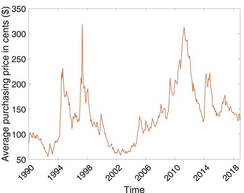
Table 1. A Comparison of Gayon et al. (2009), Karabağ and Tan (2019), and This Study.

Study	Decisions	Supply process	Production process	Demand process	Correlation between demand and supply processes
Gayon et al. (2009)	Production, pricing	Not considered	Random, capacitated	Random, price-sensitive	×
Karabağ and Tan (2019)	Procurement, production	Random	Random, capacitated	Random, governed by the market	×
This study	Procurement, production, pricing	Random	Random, capacitated	Random, price-sensitive	$✓$

Figure 2. Problem illustration.

Graphical description of the system we focus on in this study, which includes a single manufacturing facility operating in a fluctuating environment with two buffers and exponentially distributed production and raw material times.

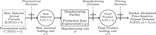
Table 2. Sets, indices, and parameters considered in the LP formulation.

$d_g$: Procurement decision, $d_g\in {\mathbb{D}}_g=\{0,1\}$	$i_1$: First inventory level, $i_1\in {\mathbb{I}}_1=\{0,1,\dots ,L_1\}$
$d_p$: Manufacturing decision, $d_p\in {\mathbb{D}}_p=\{0,1\}$	$i_2$: Second inventory level, $i_2\in {\mathbb{I}}_2=\{0,1,\dots ,L_2\}$
$d_z$: Sale price decision, $d_z\in \mathbb{D}$	e: Environment state, $e\in \mathbb{F}=\{1,2,\dots ,F\}$
$\underset{\_}{i}$: Inventory levels state, $\underset{\_}{i}\in {\mathbb{J}}^1$	${\mathbb{J}}^1$: $\left\{\right(i_1,i_2\left)\right|i_k\in {\mathbb{I}}_k\mathrm{w}\mathrm{h}\mathrm{e}\mathrm{r}\mathrm{e}k\in \{1,2\}\}$
$\mathbb{D}$: Discretised set of possible prices, $\mathbb{D}\approx {\mathcal{D}}^{\mathrm{\prime }}$	${\mathbb{J}}^2$: $\left\{\right(i_1,i_2\left)\right|i_1\in {\mathbb{I}}_1,i_2\in \left\{0\right\}\}$
${\mathbb{J}}^3$: $\left\{\right(i_1,i_2\left)\right|i_1\in {\mathbb{I}}_1,i_2\in {\mathbb{I}}_2\setminus \left\{0\right\}\}$

Table 3. The scenarios considered in the numerical analysis.

	Invariant scenario parameters				Changing scenario parameters
Scenario 1	${\delta }_H=1.25$	${\delta }_L=0.95$	$C{V}_{\overline{\delta }}=15\mathrm{\%}$	$\overline{\delta }=1.10$	$\rho \in \{-0.9,-0.8,\dots ,0.8,0.9\}$
	$c_H^g=0.90$	$c_L^g=0.30$	$C{V}_{{\overline{c}}^g}=50\mathrm{\%}$	${\overline{c}}^g=0.60$	${\mathrm{\Lambda }}_H\in \{1.05,1.10,1.15\}$
	$c^{h_1}=0.006$	$\text{β}=0.50$	$\mu =1.00$	$\overline{\mathrm{\Lambda }}=0.88$	${\mathrm{\Lambda }}_L\in \{0.70,0.65,0.60\}$
	$c^{h_2}=0.006$	$\rho =0$			$C{V}_{\overline{\mathrm{\Lambda }}}\in \{20\mathrm{\%},25\mathrm{\%},30\mathrm{\%}\}$
Scenario 2	${\mathrm{\Lambda }}_H=1.05$	${\mathrm{\Lambda }}_L=0.70$	$C{V}_{\overline{\mathrm{\Lambda }}}=20\mathrm{\%}$	$\overline{\mathrm{\Lambda }}=0.88$	$\text{β}\in \{0.50,0.52,\dots .,0.98,1.00\}$
	${\delta }_H=1.25$	${\delta }_L=0.95$	$C{V}_{\overline{\delta }}=15\mathrm{\%}$	$\overline{\delta }=1.10$	$c_H^g\in \{0.72,0.81,0.90\}$
	$c^{h_1}=0.006$	$\rho =0$	$\mu =1.00$	${\overline{c}}^g=0.60$	$c_L^g\in \{0.48,0.39,0.30\}$
	$c^{h_2}=0.006$				$C{V}_{{\overline{c}}^g}\in \{20\mathrm{\%},35\mathrm{\%},50\mathrm{\%}\}$
Scenario 3	${\mathrm{\Lambda }}_H=1.05$	${\mathrm{\Lambda }}_L=0.70$	$C{V}_{\overline{\mathrm{\Lambda }}}=20\mathrm{\%}$	$\overline{\mathrm{\Lambda }}=0.88$	$c^{h_1}\in \{0.006,0.03,0.05\}$
	${\delta }_H=1.25$	${\delta }_L=0.95$	$C{V}_{\overline{\delta }}=15\mathrm{\%}$	$\overline{\delta }=1.10$	$c^{h_2}\in \{0.006,0.03,0.05\}$
	$c_H^g=0.90$	$c_L^g=0.30$	$C{V}_{{\overline{c}}^g}=50\mathrm{\%}$	${\overline{c}}^g=0.60$	$\mu \in \{0.12,0.15,0.18,\dots ,1.5,1.53\}$
	$\text{β}=0.50$	$\rho =0$

Note: $C{V}_{{\overline{c}}^g}$, $C{V}_{\overline{\delta }}$, and $C{V}_{\overline{\mathrm{\Lambda }}}$ respectively denote the coefficients of variation for the purchasing price, the raw material inter-arrival rate, and the demand inter-arrival rate. The mathematical formulations of these coefficients are introduced in Appendix 4.

Table 4. The average time spent in environment state $e\in \{1,2,3,4\}$.

	ρ
	$-0.9$	$-0.8$	$-0.7$	$-0.6$	$-0.5$	$-0.4$	$-0.3$	$-0.2$	$-0.1$	0	0.1	0.2	0.3	0.4	0.5	0.6	0.7	0.8	0.9
$T_1$	50	50	50	50	50	50	50	50	50	50	41	33	27	21	17	13	9	6	3
$T_2$	700	450	283	200	150	117	93	75	61	50	50	50	50	50	50	50	50	50	50
$T_3$	700	450	283	200	150	117	93	75	61	50	50	50	50	50	50	50	50	50	50
$T_4$	50	50	50	50	50	50	50	50	50	50	41	33	27	21	17	13	9	6	3

Figure 3. The demand variability and correlation effects on 3(a) the average profit (α), 3(b) the average raw material inventory level ($\mathrm{E}\left[i_1\right]$), 3(c) the average final product inventory level ($\mathrm{E}\left[i_2\right]$), and 3(d) the average price ($\mathrm{E}\left[s\right]$).

3(a) For three different levels of demand variability, these line graphs show how the average profit changes as the correlation coefficients vary between -1 and 1, 3(b) For three different levels of demand variability, these line graphs show how the average raw material level changes as the correlation coefficients vary between -1 and 1, 3(c) For three different levels of demand variability, these line graphs show how the average final product level changes as the correlation coefficients vary between -1 and 1, 3(d) For three different levels of demand variability, these line graphs show how the average price changes as the correlation coefficients vary between -1 and 1.

Figure 4. The price sensitivity and procurement price variability effects on 4(a) the average profit (α), 4(b) the average raw material inventory level ($\mathrm{E}\left[i_1\right]$), 4(c) the average final product inventory level ($\mathrm{E}\left[i_2\right]$), and 4(d) the average price ($\mathrm{E}\left[p\right]$).

4(a) For three different levels of price variability, these line graphs show how the average profit changes as the price sensitivity levels vary between 0.5 and 1, 4(b) For three different levels of price variability, these line graphs show how the average raw material level changes as the price sensitivity levels vary between 0.5 and 1, 4(c) For three different levels of price variability, these line graphs show how the average final product level changes as the price sensitivity levels vary between 0.5 and 1, 4(d) For three different levels of price variability, these line graphs show how the average price changes as the price sensitivity levels vary between 0.5 and 1.

Figure 5. The production rate and holding cost effects on 5(a) the average profit (α), 5(b) the average raw material inventory level ($\mathrm{E}\left[i_1\right]$), 5(c) the average final product inventory level ($\mathrm{E}\left[i_2\right]$), and 5(d) the average price ($\mathrm{E}\left[p\right]$).

5(a) For three different levels of holding cost, these line graphs show how the average profit changes as the production rate varies between 0.12 and 1.53, 5(b) For three different levels of holding cost, these line graphs show how the average raw material level changes as the production rate varies between 0.12 and 1.53, 5(c) For three different levels of holding cost, these line graphs show how the average final product level changes as the production rate varies between 0.12 and 1.53, 5(d) For three different levels of holding cost, these line graphs show how the average price changes as the production rate varies between 0.12 and 1.53.

Figure 6. The demand variability and correlation effects on the relative difference between dynamic and static pricing strategies.

For three different levels of demand variability, this line graph depicts the profit improvement of using dynamic pricing relative to static pricing as the correlation coefficient varies between -1 and 1.

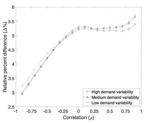
Figure 7. The price sensitivity and procurement price variability effects on the relative difference between dynamic and static pricing strategies.

For three different levels of price variability, this line graph depicts the profit improvement of using dynamic pricing relative to static pricing as the price sensitivity level varies between 0.5 and 1.

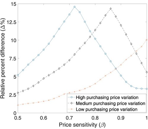
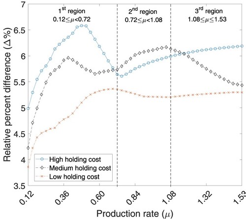
Figure 8. Effects of production rate and holding cost on the relative difference between dynamic and static pricing strategies.

For three different levels of holding cost, this line graph depicts the profit improvement of using dynamic pricing relative to static pricing as the production rate varies between 0.12 and 1.53.

Gayon, J.-P., I. Talay-Değirmenci, F. Karaesmen, and E. L. Örmeci. 2009. “Optimal Pricing and Production Policies of a Make-to-Stock System with Fluctuating Demand.” Probability in the Engineering and Informational Sciences 23 (2): 205–230.

 Web of Science ®Google Scholar

Karabağ, O., and B. Tan. 2019. “Purchasing, Production, and Sales Strategies for a Production System with Limited Capacity, Fluctuating Sales and Purchasing Prices.” IISE Transactions 51 (9): 921–942.

 Web of Science ®Google Scholar

Data availability statement

Data sharing is not applicable to this article as no new data were created or analysed in this study.