Emergency medical supplies scheduling during public health emergencies: algorithm design based on AI techniques

Figures & data

Table 1. Emergency supplies dispatch table.

Optimisation mode	Target	Method	References	Whether to consider fairness and justice
Single object optimisation	Minimum rescue time	Genetic algorithm and analytic hierarchy process	Wan, Ye, and Peng (2023)	No
		Genetic algorithm	Chang et al. (2023a)	No
	Shortest distance	Particle swarm optimisation and a genetic algorithm	Deng et al. (2023)	No
		Discrete artificial bee colony algorithms	Wang, Zhao, and Wu (2023)	No
Multi-objective optimisation	minimising driving distance, reducing delay time, and optimising vehicle utilisation	Ant colony optimisation and genetic algorithm	Lopes et al. (2022)	No
		The Greedy randomised adaptive search procedure	Fernández Gil et al. (2023)	No
		An adaptive augmented ε-constraint method	Gao et al. (2021)	Yes

Table 2. The parameter list.

Parameter type	Parameter	Define
Model parameter	$c_{ijr}$	The minimum distance of vehicle r from demand point i to j
	$S_r$	Fixed vehicle speed
	$s_i$	Quantity delivered at disaster site i
	$d_i$	Quantity demanded at disaster site i
	$M_r$	Maximum capacity of vehicle r
	C	Set of disaster sites, C = i| i = 1, 2, … , N
	B	Set of distribution centre, B = b| b = 1, 2, … , M
	V	Emergency vehicle set, v = r | r = 1, 2, … , K
	N	All nodes in the transportation network, N = B ∪ C
	$Q_b$	Amount of medical supplies in distribution centre b
	${\gamma }_i$	The priority of demand point i
	θ	The efficiency parameter of the vehicle, that is, the amount of material loaded per unit of time
	$C_1$	Penalty cost per unit time for arrivals beyond the latest tolerance time
	T	$T=\left(s_1,s_2,\dots ,s_n\right)$ represents the emergency supplies allocation amount
Intermediate variable parameters	$T_r^i$	The point in time when vehicle r arrives at demand point i, $T_r^i=0$ means the vehicle starting from the distribution centre
	$t_{ijr}$	The travelling time of vehicle r from demand point i to demand point j, $t_{ijr}={\displaystyle \frac{c_{ijr}}{V_r}}$
	${t_{ir}}^{\mathrm{\prime }}$	Vehicle r demand point I service time, $t_{ir}^{\mathrm{\prime }}={\displaystyle \frac{s_i}{\theta }}$
	$w_i$	The satisfaction rate of demand point i, $w_i={\displaystyle \frac{s_i}{d_i{\gamma }_i}}$
	$z_{ijr}$	When vehicle r and distribution centre i transport supplies to distribution centre j, $i,j\in B$, then $z_{ijr}=1,$otherwise $z_{ijr}=0$

Figure 1. Reinforcement learning mechanism.

The pheromone communication is carried out between population A and population B, and the Markov dynamic decision judgment of reinforcement learning is used to reward or punish population A or population B.

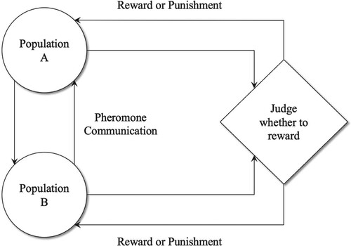
Figure 2. Location distribution diagram of the example: (a) Example R101: (b) Example C101.

Figures (a) and (b) show the location distribution of 24 suppliers’ demand points and 3 distribution centres in the R101 and C101.

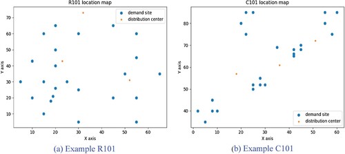
Table 3. R101 example demand point information table.

Demand point number	X coordinates (km)	Y coordinates (km)	Demand quantity (units)	Latest service time $l_i$ (min)	Latest tolerance time $l{l}_i$ (min)
1	55	45	13	116	126
2	55	20	19	149	159
3	15	30	26	34	44
4	25	30	3	99	109
5	20	50	5	81	91
6	10	43	9	95	105
7	55	60	16	97	107
8	30	60	16	124	134
9	20	65	12	67	77
10	50	35	19	63	73
11	30	25	23	159	169
12	15	10	20	32	42
13	30	5	8	61	71
14	10	20	19	75	85
15	5	30	2	157	167
16	20	40	12	87	97
17	15	60	17	76	86
18	45	65	9	126	136
19	45	20	11	62	72
20	55	5	29	68	78
21	65	35	3	153	163
22	18	18	17	185	195
23	20	26	9	83	93
24	19	21	10	58	68

Table 4. R101 example distribution centre information table.

Distribution centre number	X coordinates	Y coordinates	Material total
1	23	43	60
2	32	73	80
3	52	31	110

Table 5. R101 example distribution vehicle information table.

Type of delivery vehicle	Maximum capacity (units)	Ground speed (km/min)	Vehicle efficiency parameters (units/min)
1	50	1	8
2	30	1	5

Table 6. C101 example demand point information table.

Demand point number	X coordinates (km)	Y coordinates (km)	Demand quantity (units)	Latest service time $l_i$ (min)	Latest tolerance time $l{l}_i$ (min)
1	45	68	10	912	967
2	45	70	30	825	870
3	42	66	10	65	146
4	42	68	10	727	782
5	42	65	10	15	67
6	35	69	10	448	505
7	25	85	20	652	721
8	22	75	30	30	92
9	22	85	10	567	620
10	20	80	40	384	429
11	10	40	30	31	100
12	8	40	40	87	158
13	8	45	20	751	816
14	5	35	10	283	344
15	2	40	20	383	716
16	30	52	20	914	965
17	28	52	20	812	883
18	28	55	10	732	777
19	25	50	10	65	144
20	25	52	40	169	224
21	60	85	30	561	622
22	58	75	20	30	84
23	55	80	10	743	820
24	55	85	20	647	726

Table 7. C101 example distribution centre information table.

Distribution centre number	X coordinates	Y coordinates	Material total
1	40	50	80
2	26	33	110
3	52	21	170

Table 8. C101 example distribution vehicle information table.

Type of delivery vehicle	Maximum capacity (units)	Ground speed (km/min)	Vehicle efficiency parameters (units/min)
1	60	1	15
2	50	1	10

Figure 3. Iteration diagram of fair index optimisation: (a) R101 iterative graph of fair index optimisation: (b) C101 iterative graph of fair index optimisation.

In Figure (a), the fairness index of example R101 tends to converge after about 100 iterations, and the convergence value is 0.083; In Figure (b), the fairness index of C101 example converges in about 230 iterations, and the convergence value is 0.054.

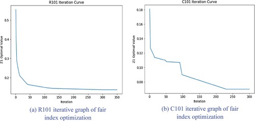
Figure 4. Ant colony parameter tuning: (a) ACS algorithm and parameter: (b) MMAS algorithm and parameter: (c) ACS algorithm parameter selection: (d) MMAS algorithm parameter selection: (e) Ant Quantity.

In Figure (a), the ACS algorithm is used to obtain the optimal α and β factors, where α = 2, β = 5.5; In Figure (b), the MMAS algorithm is used to obtain the optimal α and β factors, where α = 2.5, β = 5; In Figure (c), the ACS algorithm is used to screen ρ, and the optimal ρ = 0.2; Figure (d) uses the MMAS algorithm to screen ρ, and the optimal ρ = 0.8; Figure (e) compares the number of ants of 12,16,24,30,36, the optimal objective function is the best, and the number of ants that converges the fastest is 24.

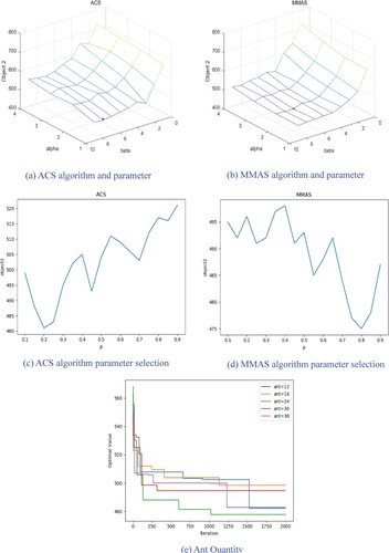
Figure 5. Roadmap of vehicle distribution: (a) R101 Vehicle distribution roadmap: (b) C101 Vehicle distribution roadmap.

Figure (a) shows the optimal vehicle assignment route of the R101 example, as shown in Table 9; Figure (b) shows the optimal vehicle assignment route for the C101 example, as shown in Table 10.

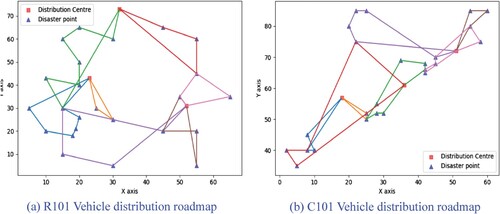
Table 9. R101 is an example of a vehicle distribution route.

Distribution centre	Vehicle number	Distribution line
1	1,2	(15,14,22,24,23,3),(4,11)
2	3,4	(8,9,17,5,16,6,3),(18,7,1)
3	5,6,7	(13,12,3,11,19),(20,2,19,10),(10,1,21)

Table 10. C101 is an example of a vehicle distribution route.

Distribution centre	Vehicle number	Distribution line
1	1,2	(13,11,12),(20,19)
2	3,4	(16,17,19,18,6,4,3),(14,15,12,8)
3	5,6,7	(8,10,9,7,2),(24,21,23),(5,3,1,2,23,22)

Table 11. Comparison of the results of two allocation schemes.

Solution result	Priority is considered	Priority is not considered
R101 Dispatch time	531	522
R101 Penalty costs	1020	1760
C101 Dispatch time	377	380
C101 Penalty costs	440	690

Table 12. R101 example algorithm comparison results.

Evaluation index	The algorithm in this paper	Traditional genetic algorithm
Objective function $Z_1$	0.083	0.087
Convergent iteration number	300	456
Run time	218 s	240 s

Table 13. C101 example algorithm comparison results.

Evaluation index	The algorithm in this paper	Traditional genetic algorithm
Objective function $Z_1$	0.054	0.063
Convergent iteration number	500	527
Run time	203 s	224 s

Figure 6. Comparison of algorithm convergence: (a) Comparison of algorithm convergence in R101 example: (b) Comparison of algorithm convergence in C101 example.

Figures (a) and (b) show the comparison between the ACS-MMAS, ACS, and MMAS algorithms for R101 and C101 examples, respectively. The results show that the Z2 value obtained by the ACS-MMAS algorithm is smaller than that obtained by ACS and MMAS algorithms.

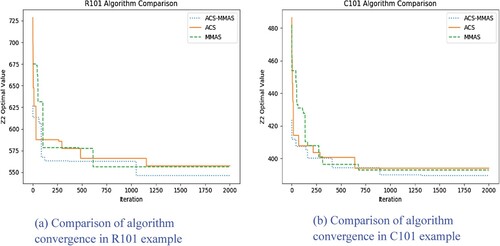
Figure 7. Pareto frontier comparison of algorithms: (a) R101 example Pareto frontier: (b) C01 example Pareto frontier.

Figure (a) and Figure (b) respectively show that the ACS-MMAS algorithm is used to obtain more Pareto solution sets on the pre-Pareto curve for R101 and C101 examples, and the controllable space is larger than the ACS algorithm and MMAS algorithm.

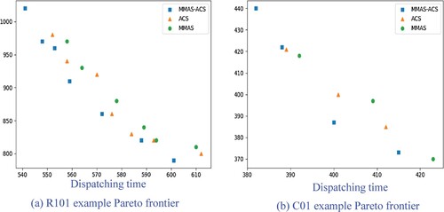
Figure 8. Shadow area is the HV value of the solution set S′.

a1, a2 a3 are the three Pareto solutions, and the hypervolume value is the sum of the volumes of the hypervolume cube.

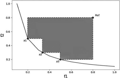
Table 14. Algorithm HV value comparison.

Example/ Algorithm	ACS algorithm	MMAS algorithm	ACS-MMAS algorithm
R101	0.698	0.712	0.731
C101	0.725	0.737	0.754

Wan, M., C. Ye, and D. Peng. 2023. “Multi-period Dynamic Multi-Objective Emergency Material Distribution Model Under Uncertain Demand.” Engineering Applications of Artificial Intelligence 117: 105530. 11.top/10.1016j.engappai.2022.105530.

 Web of Science ®Google Scholar

Chang, K. H., T. L. Chen, F. H. Yang, and T. Y. Chang. 2023a. “Simulation Optimization for Stochastic Casualty Collection Point Location and Resource Allocation Problem in a Mass Casualty Incident.” European Journal of Operational Research 309 (3): 1237–1262. https://doi.org/10.1016/j.ejor.2023.01.065

 Web of Science ®Google Scholar

Deng, J., X. Chen, W. Wei, and J. Liang. 2023. “Resource Coordination Scheduling Optimisation of Logistics Information Sharing Platform Considering Decision Response and Competition.” Computers & Industrial Engineering 176: 108892. 11.top/10.1016j.cie.2022.108892.

 Web of Science ®Google Scholar

Wang, L., X. Zhao, and P. Wu. 2023. “Large-scale Emergency Medical Services Scheduling During the Outbreak of Epidemics.” Annals of Operations Research 39: 1–25. https://doi.org/10.1007/s10479-023-05218-4.

 Google Scholar

Lopes, T. C., A. S. Michels, N. Brauner, and L. Magatão. 2022. “Balancing-sequencing Paced Assembly Lines: A Multi-Objective Mixed-Integer Linear Case Study.” International Journal of Production Research 61 (17): 5901–5917. https://doi.org/10.1080/00207543.2022.2118888.

 Web of Science ®Google Scholar

Fernández Gil, A., E. Lalla-Ruiz, M. Gómez Sánchez, and C. Castro. 2023. “The Cumulative Vehicle Routing Problem with Time Windows: Models and Algorithm.” Annals of Operations Research  39: 1–29. https://doi.org/10.1007/s10479-022-05102-7.

 Google Scholar

Gao, X., X. Jin, P. Zheng, and C. Cui. 2021. “Multi-modal Transportation Planning for Multi-Commodity Rebalancing Under Uncertainty in Humanitarian Logistics.” Advanced Engineering Informatics 47: 101223. 11.top/10.1016j.aei.2020.101223.

 Web of Science ®Google Scholar

Data availability statement

Data available on request from the authors.