A multi-domain mixture density network for tool wear prediction under multiple machining conditions

Figures & data

Figure 1. (a) Conventional approaches and (b) the proposed approach to multi-domain tool wear prediction.

(a) Multiple models take distinct input signals individually and each of them outputs tool wear prediction. (b) Diverse input signals are fed into the proposed model (i.e. MD2N) at once and are transformed into predicted tool wear.

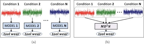
Figure 2. MD${}^2$N: the proposed model architecture.

The experimental setup using multiple machining conditions that generate multivariate time-series input signals, leading to the Bayesian domain-invariant feature extractor that consists of multiple neural network layers, leading to the mixture density network and the auxiliary domain classifier, simultaneously.

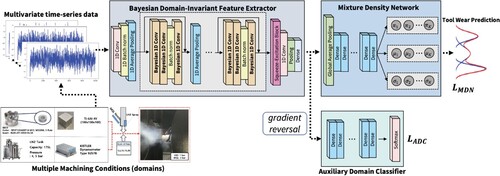
Figure 3. The detailed architectural structure of BDIFE.

A series of neural network layers stacked and connected with arrows in an order that constitutes the proposed BDIFE architecture.

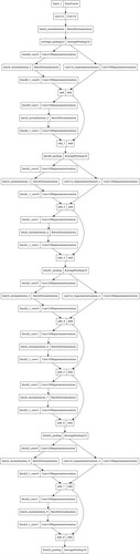
Figure 4. The experimental setup for the milling process.

The cutting tool and tool holder attached to the work material, performing a milling process with a dynamometer attached to the work stage, the lubricant nozzle facing toward the cutting tool.

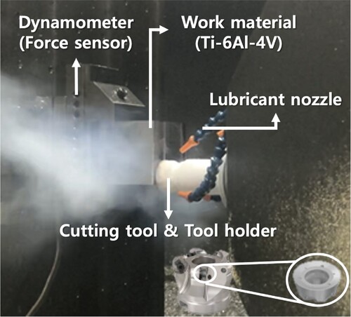
Figure 5. The schematic diagram of the experimental setup.

The 5-axis CNC machine with the work stage positioned on left with other experimental settings, leading to the measurement of tool wear and data acquisition, leading to a PC that inputs tool wear length and cutting force.

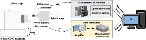
Table 1. Milling experiment conditions.

Experiment number	Setting	Cutting speed (m/min)	Feed (mm/tooth)	Axial depth (mm)	Radial depth (mm)	Material removal rate (${\mathrm{m}\mathrm{m}}^3/min$)	Number of pass
1	Wet	60	0.6	1.0	18.0	5490.0	[1,5,10,15,20]
2	Wet	80	0.6	1.0	18.0	5500.0
3	Wet	60	0.8	1.0	18.0	5500.0
4	Wet	60	0.6	1.3	18.0	5363.0
5	CryoMQL	60	0.6	1.0	18.0	5490.0
6	CryoMQL	80	0.6	1.0	18.0	5500.0
7	CryoMQL	60	0.8	1.0	18.0	5500.0
8	CryoMQL	60	0.6	1.3	18.0	5363.0

Table 2. Descriptive statistics of datasets.

	Dataset 1			Dataset 2			Dataset 3			Dataset 4
Number Variable	$F_x$	$F_y$	$F_z$	$F_x$	$F_y$	$F_z$	$F_x$	$F_y$	$F_z$	$F_x$	$F_y$	$F_z$
Mean	81.0290	45.0864	64.7218	78.1679	44.0454	103.4832	95.0169	54.7226	106.5160	96.7278	53.5007	108.3236
SD	225.7679	112.8530	132.1324	232.5850	111.3457	153.2089	284.9614	144.2577	176.5907	283.6351	142.5736	168.3237
Min	−496.0630	−406.0360	−52.4902	−640.8690	−447.6930	−50.3540	−494.8430	−544.2810	−56.4575	−450.8970	−517.2730	−53.7109
Max	2102.0500	1121.2200	711.6700	2129.0600	1027.9800	823.3640	2738.4900	1344.4500	1087.6500	2629.3900	1323.5500	979.6140
	Dataset 5			Dataset 6			Dataset 7			Dataset 8
Number Variable	$F_x$	$F_y$	$F_z$	$F_x$	$F_y$	$F_z$	$F_x$	$F_y$	$F_z$	$F_x$	$F_y$	$F_z$
Mean	80.0653	46.7010	−38.4820	82.0602	45.2524	1.4938	92.2392	55.6570	−52.6978	101.0826	53.7894	−83.4370
SD	228.4289	123.2950	147.1831	231.0209	117.2994	169.6341	264.6479	146.0505	159.0441	282.8738	146.6253	186.6293
Min	−519.8670	−456.0850	−232.8490	−637.0540	−456.6960	−217.5900	−439.9110	−550.2320	−257.8740	−729.2180	−618.2860	−358.5820
Max	2104.8000	1231.2300	689.0870	2107.2400	1193.0800	773.3150	2536.3200	1419.0700	847.1680	2671.8100	1533.9700	810.8520

Figure 6. Visualisation of sensor measurements.

A plot of three force signals in the x, y, and z directions, each coloured with different colours, with the x-axis of time measured in milliseconds and the y-axis of the force measured in Newton.

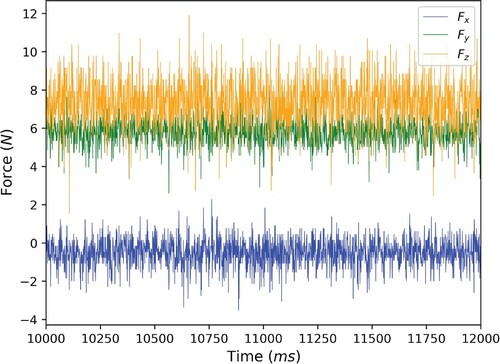
Figure 7. Measured tool wear of (a) Experiment 2 and (b) Experiment 6.

Actual measurement of the surface of work material in wet and CryoMQL settings at 1, 5, 10, 15, and 20 passes positioned from top to bottom, the crack and wear progress as the machining proceeds.

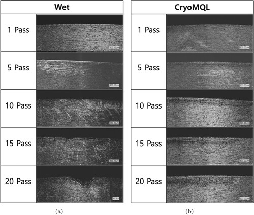
Table 3. Prediction performance for wet and CryoMQL setting data.

		Metric
Setting	Test dataset	MAE	RMSE	MAPE
Wet	1	2.6772	6.7216	0.0637
		(±0.4948)	(±0.9715)	(±0.0117)
	2	2.6201	5.0101	0.0437
		(±0.4353)	(±0.7046)	(±0.0082)
	3	5.3429	9.0277	0.0699
		(±1.1129)	(±1.0737)	(±0.0132)
	4	3.4466	6.7388	0.0466
		(±0.3091)	(±0.8121)	(±0.0041)
	All (1 + 2 + 3 + 4)	3.5198	7.1057	0.0570
		(±0.3430)	(±0.5456)	(±0.0061)
CryoMQL	5	1.2266	2.2234	0.0235
		(±0.1676)	(±0.4135)	(±0.0032)
	6	1.3638	3.3404	0.0328
		(±0.5127)	(±0.3822)	(±0.0130)
	7	3.4514	5.7562	0.0476
		(±2.1667)	(±1.7699)	(±0.0278)
	8	1.1237	2.5992	0.0182
		(±0.4187)	(±0.1322)	(±0.0064)
	All (5 + 6 + 7 + 8)	1.7204	3.6470	0.0292
		(±0.7231)	(±0.6684)	(±0.0111)

Table 4. Prediction performance for both settings data.

	Metric
Test dataset	MAE	RMSE	MAPE
1	1.7139	3.7887	0.0374
	(±0.4186)	(±0.3156)	(±0.0032)
2	2.6190	5.2913	0.0452
	(±0.5090)	(±0.8235)	(±0.0103)
3	4.1183	6.5092	0.0512
	(±0.5812)	(±0.7506)	(±0.0025)
4	4.4241	9.9750	0.0559
	(±0.6486)	(±1.3586)	(±0.0079)
5	1.4735	3.8300	0.0237
	(±0.3564)	(±0.6313)	(±0.0050)
6	1.8446	5.6408	0.0428
	(±0.5028)	(±1.0257)	(±0.0115)
7	3.3007	6.1715	0.0402
	(±0.7133)	(±1.4229)	(±0.0063)
8	1.2603	3.8236	0.0199
	(±0.1647)	(±0.4435)	(±0.0027)
All (1∼8)	2.1748	5.6422	0.0350
	(±0.2655)	(±0.6205)	(±0.0041)

Figure 8. Tool wear prediction performance of MD${}^2$N on all datasets under wet and CryoMQL settings. (a) Dataset 1. (b) Dataset 2. (c) Dataset 3. (d) Dataset 4. (e) Dataset 5. (f) Dataset 6. (g) Dataset 7 and (h) Dataset 8.

Tool wear prediction results with an increasing plot with a black solid line for the ground-truth tool wear and a coloured line for the predicted tool wear for every dataset, the x-axis represents machining distances measured in millimetres and the y-axis showing tool wear degrees measured in micrometres.

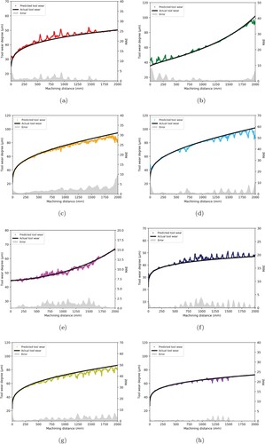
Figure 9. t-SNE visualisation of the latent space of MD${}^2$N: (a) before training, (b) after 100 epochs, (c) after 200 epochs, (d) after 300 epochs, and (e) after training.

Two-dimensional visualisation of the latent space generated using the proposed method, scatterplots with each point representing a data sample, each sampled coloured differently according to the machining setting.

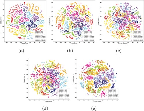
Table 5. Performance comparison with existing models.

	Wet			CryoMQL			Wet + CryoMQL
Dataset Model	MAE	RMSE	MAPE	MAE	RMSE	MAPE	MAE	RMSE	MAPE
SVR	17.6989	22.2290	0.2897	11.0229	13.0161	0.1928	14.3869	16.8103	0.2570
	(±0.0795)	(±0.0869)	(±0.0003)	(±0.0561)	(±0.0976)	(±0.0010)	(±0.0297)	(±0.0310)	(±0.0005)
RF	11.0783	15.3236	0.1947	7.1514	10.2964	0.1230	9.6556	13.2919	0.1681
	(±0.0344)	(±0.0381)	(±0.0005)	(±0.0211)	(±0.0281)	(±0.0004)	(±0.0269)	(±0.0313)	(±0.0002)
LSTM	11.1720	13.7242	0.2730	6.4884	8.6648	0.1134	7.8924	10.4880	0.1368
	(±1.1396)	(±1.2325)	(±0.1679)	(±1.4033)	(±1.1930)	(±0.0276)	(±1.1525)	(±0.9437)	(±0.0201)
GRU	9.2271	11.9802	0.1589	5.9730	8.2016	0.1028	7.7760	10.5061	0.1339
	(±0.8675)	(±0.6444)	(±0.0133)	(±0.5707)	(±0.5442)	(±0.0101)	(±1.9583)	(±1.9467)	(±0.0335)
CNN	16.5959	18.8952	0.2875	9.9452	11.5631	0.1811	13.6391	16.3143	0.2187
	(±0.0824)	(±0.0584)	(±0.0013)	(±0.0307)	(±0.0085)	(±0.0011)	(±0.0451)	(±0.0499)	(±0.0465)
MD${}^2$N (proposed)	3.5198	7.1057	0.0570	1.7204	3.6470	0.0292	2.1748	5.6422	0.0350
	(±0.3430)	(±0.5456)	(±0.0061)	(±0.7231)	(±0.6684)	(±0.0111)	(±0.2655)	(±0.6205)	(±0.0041)

Table 6. Performance comparison with state-of-the-art methods.

	Wet			CryoMQL			Wet + CryoMQL
Dataset Model	MAE	RMSE	MAPE	MAE	RMSE	MAPE	MAE	RMSE	MAPE
J. Wang et al. (2019)	17.4631	18.6138	0.2669	11.0320	12.8133	0.2032	14.0741	16.6116	0.2471
	(±0.4771)	(±2.6608)	(±0.0550)	(±0.0352)	(±0.0355)	(±0.0008)	(±0.0243)	(±0.0260)	(±0.0004)
Sun et al. (2020)	10.4252	13.0826	0.1857	6.8283	8.9031	0.1191	7.7869	10.4658	0.1372
	(±0.6919)	(±0.6727)	(±0.0173)	(±0.3657)	(±0.3557)	(±0.0070)	(±0.5893)	(±0.6665)	(±0.0099)
Hahn and Mechefske (2021)	9.5482	12.2764	0.1653	5.9108	8.1009	0.1020	7.4294	10.2782	0.1290
	(±0.1381)	(±0.0980)	(±0.0040)	(±0.2353)	(±0.1691)	(±0.0045)	(±0.1579)	(±0.1713)	(±0.0027)
MD${}^2$N (proposed)	3.5198	7.1057	0.0570	1.7204	3.6470	0.0292	2.1748	5.6422	0.0350
	(±0.3430)	(±0.5456)	(±0.0061)	(±0.7231)	(±0.6684)	(±0.0111)	(±0.2655)	(±0.6205)	(±0.0041)

Wang, Jinjiang, Jianxing Yan, Chen Li, Robert X. Gao, and Rui Zhao. 2019. “Deep Heterogeneous GRU Model for Predictive Analytics in Smart Manufacturing: Application to Tool Wear Prediction.” Computers in Industry 111:1–14. https://doi.org/10.1016/j.compind.2019.06.001.

 Web of Science ®Google Scholar

Sun, Huibin, Jiduo Zhang, Rong Mo, and Xianzhi Zhang. 2020. “In-Process Tool Condition Forecasting Based on a Deep Learning Method.” Robotics and Computer-Integrated Manufacturing 64:101924. https://doi.org/10.1016/j.rcim.2019.101924.

 Web of Science ®Google Scholar

Hahn, Tim Von, and Chris K. Mechefske. 2021. “Self-Supervised Learning for Tool Wear Monitoring with a Disentangled-Variational-Autoencoder.” International Journal of Hydromechatronics 4 (1): 69–98. https://doi.org/10.1504/IJHM.2021.114174.

 Google Scholar

Data availability statement

The data that support the findings of this work are available from the corresponding author, [SL], upon reasonable request.