Views

CrossRef citations to date

Altmetric

Research Articles

Adaptive population-based simulated annealing for resource constrained job scheduling with uncertainty

Dhananjay Thiruvadya School of Information Technology, Deakin University, Geelong, AustraliaCorrespondence[email protected]

https://orcid.org/0000-0002-8011-933X View further author information

Su Nguyenb School of Accounting, Information Systems and Supply Chain, RMIT University, Melbourne, AustraliaView further author information

Yuan Sunc La Trobe Business School, La Trobe University, Melbourne, AustraliaView further author information

Fatemeh Shirid Faculty of Information Technology, Monash University, Melbourne, AustraliaView further author information

Nayyar Zaidia School of Information Technology, Deakin University, Geelong, AustraliaView further author information

Xiaodong Lie School of Science, RMIT University, Melbourne, AustraliaView further author information

Figures & data

Table 1. An example with 3 jobs and 10 units of resource.

Download CSV Display Table

Figure 1. An example that demonstrates job swapping. Two indices are selected randomly, and the corresponding jobs are swapped. In this example, indices 3 and 9 are selected, and the jobs within those indices, 2 and 9, are swapped.

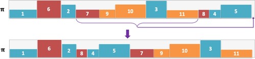
Image of sequence of jobs, followed by applying β-sampling. Five jobs, starting at position 4, are moved to the end of the sequence.

Figure 2. An example that demonstrates β-sampling. From the sequence π, a subset of jobs is selected (7, 9, 10, 3, 11) and moved to the end of the sequence.

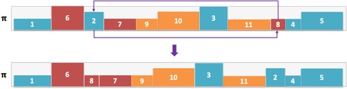
Image of sequence of jobs, followed by applying job swapping. Jobs at position 3 and 9, are swapped.

Figure 3. Adaptive probabilities over 200 simulations.

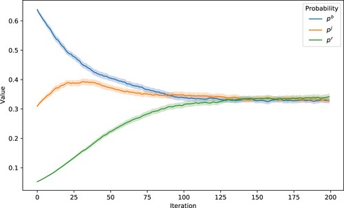
The convergence profile of of the three adaptive probabilities, pb, pj and pr. We see that all the probabilities converge to approximately 1/3.

Figure 4. An example of a problem with three machines and 15 jobs. From π, jobs are selected in order (left to right) and scheduled on machines that they belong to (e.g. orange jobs on $m_{2}$ ). Those jobs that have predecessors that are not yet scheduled will be put on the waiting list $\hat{π}$ ; (a) Job 8 requires Job 2 to be scheduled before it can be scheduled. (b) Job 8 is scheduled once Job 2 has been scheduled, and this will be done as early as possible considering resources.

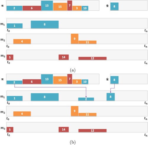
(a) The figure shows a partial sequence of jobs (π), a waiting list (π^) and three machines (m1,m2,m3). Jobs of the same colour go on the same machine, e.g. blue jobs on machine m1. (b) Job 2 is placed on machine m1 at the first time point where the resources are available. Following this, Job 8 on the waiting list is released, and is also placed in the first available time point on machine m1.

Table 2. Results of ACS, SACS and APSA shown as the percentage difference to the best solution for uncertainty levels 0.5, 0.6 and 0.7; Results in column ‘Best’ are highlighted in bold if APSA finds the best solution; Results for each algorithm are highlighted in bold when they achieve best average results, while statistically significant results (pair-wise Wilcoxon ranked-sum test) at a 95 $%$ confidence interval are marked with a *.

Display Table

Table 3. Results of ACS, SACS and APSA shown as the percentage difference to the best solution for uncertainty levels 0.8, 0.9 and 1.0; Results in column ‘Best’ are highlighted in bold if APSA finds the best solution; Results for each algorithm are highlighted in bold when they achieve best average results, while statistically significant results (pair-wise Wilcoxon ranked-sum test) at a 95 $%$ confidence interval are marked with a *.

Display Table

Figure 5. The figure shows a bar chart of the performance of ACS, SACS and APSA. It shows the average percentage difference to best (y-axis) for each uncertainty level (x-axis). We see that APSA has a distinct advantage across all uncertainty levels.

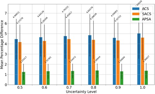
A comparison of ACS, SACS and APSA across six uncertainty levels. There is a clear advantage of APSA over the other two methods.

Figure 6. A comparison of SACS (left) and APSA (right) for RCJSU at uncertainty level 0.6 considering varying levels of resource utilisation (top = 0.25 $%$ , middle = 0.5 $%$ , bottom = 0.75 $%$ ), machine sizes and precedence proportion. Gap $%$ = $(B - b^{*}) / b^{*}$ , where B is APSA or SACS and b* is the best solution.

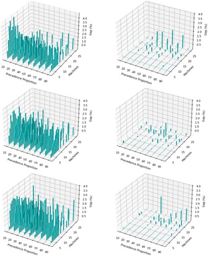
A comparison of SACS and APSA considering problem characteristics including precedence proportion, resource utilisation and number of machines for uncertainty level 0.6.

Figure 7. A comparison of SACS (left) and APSA (right) for RCJSU at uncertainty level 0.9 considering varying levels of resource utilisation (top = 0.25 $%$ , middle = 0.5 $%$ , bottom = 0.75 $%$ ), machine sizes and precedence proportion. Gap $%$ = $(B - b^{*}) / b^{*}$ , where B is APSA or SACS and $b^{*}$ is the best solution.

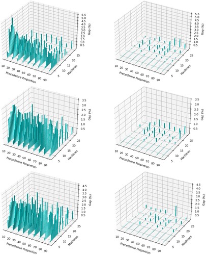
A comparison of SACS and APSA considering problem characteristics including precedence proportion, resource utilisation and number of machines for uncertainty level 0.9. There is a clear advantage for APSA on small and medium sized problems and a small advantage on large problems.

Figure 8. Convergence profiles of ACS, SACS and APSA on four RCJSU problem instances of different sizes. The instances chosen are 3–53, 6–28, 9–47 and 12–14. The TWTs on the y-axes are presented on a logarithmic scale.

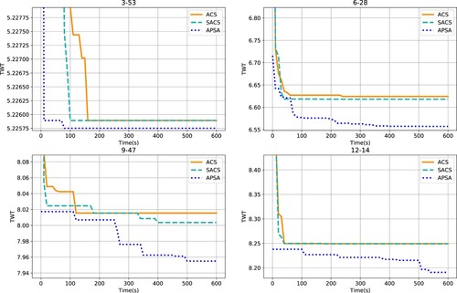
Each figure compares ACS, SACS and APSA for a single run for the problem instances 3–53, 6–28, 9–47 and 12–14. We see how APSA is able to find higher quality solutions early, and due to the adaptive probabilities, it is able to continue to improve across a run for all problem instances.

Table 4. A comparison of APSA and the original SA (Singh and Ernst Citation2011) (OSA) for the uncertainty levels of 0.6 and 0.9; Results for each algorithm are highlighted in bold when they achieve best average results, while statistically significant results (pair-wise Wilcoxon ranked-sum test) at a 95 $%$ confidence interval are marked with a *.

Display Table

Table 5. A comparison of APSA with different population sizes, v = 10 and v = 1, on the problem instances with uncertainty levels of 0.6 and 0.9; Results for each algorithm are highlighted in bold when they achieve best average results, while statistically significant results (pair-wise Wilcoxon ranked-sum test) at a 95 $%$ confidence interval are marked with a *.

Display Table

Table 6. A comparison of CGACO (Thiruvady, Singh, and Ernst Citation2014), ACS, SACS and APSA on RCJS.

Display Table

Table A1. A comparison of APSA variants with different population sizes, $v \in {1, 5, 10, 20}$ , on selected problem instances (4–61, 8–53, 12–14 and 20–6) with uncertainty levels of 0.6 and 0.9.

Display Table

Table A2. A comparison of APSA variants with different levels of Metropolis-Hastings iterations, $Iter \in 1000, 2500, 5000, 10, 000$ , on selected problem instances (4–61, 8–53, 12–14 and 20–6) with uncertainty levels of 0.6 and 0.9.

Display Table

Table A3. A comparison of APSA variants with different levels of γ, $γ \in 0.2, 0.5, 0.8, 0.95$ , on selected problem instances (4–61, 8–53, 12–14 and 20–6) with uncertainty levels of 0.6 and 0.9.

Display Table

Data availability statement

The authors confirm that the data supporting the findings of this study are available within the article.

Adaptive population-based simulated annealing for resource constrained job scheduling with uncertainty

Table 1. An example with 3 jobs and 10 units of resource.

Table 6. A comparison of CGACO (Thiruvady, Singh, and Ernst Citation2014), ACS, SACS and APSA on RCJS.

Table A1. A comparison of APSA variants with different population sizes, $v \in {1, 5, 10, 20}$ , on selected problem instances (4–61, 8–53, 12–14 and 20–6) with uncertainty levels of 0.6 and 0.9.

Table A2. A comparison of APSA variants with different levels of Metropolis-Hastings iterations, $Iter \in 1000, 2500, 5000, 10, 000$ , on selected problem instances (4–61, 8–53, 12–14 and 20–6) with uncertainty levels of 0.6 and 0.9.

Table A3. A comparison of APSA variants with different levels of γ, $γ \in 0.2, 0.5, 0.8, 0.95$ , on selected problem instances (4–61, 8–53, 12–14 and 20–6) with uncertainty levels of 0.6 and 0.9.

Information for

Open access

Opportunities

Help and information

Your download is now in progress and you may close this window

Login or register to access this feature

Adaptive population-based simulated annealing for resource constrained job scheduling with uncertainty

Figures & data

Table 1. An example with 3 jobs and 10 units of resource.

Table 6. A comparison of CGACO (Thiruvady, Singh, and Ernst Citation2014), ACS, SACS and APSA on RCJS.

Table A1. A comparison of APSA variants with different population sizes, v∈{1,5,10,20}, on selected problem instances (4–61, 8–53, 12–14 and 20–6) with uncertainty levels of 0.6 and 0.9.

Table A2. A comparison of APSA variants with different levels of Metropolis-Hastings iterations, Iter∈1000,2500,5000,10,000, on selected problem instances (4–61, 8–53, 12–14 and 20–6) with uncertainty levels of 0.6 and 0.9.

Table A3. A comparison of APSA variants with different levels of γ, γ∈0.2,0.5,0.8,0.95, on selected problem instances (4–61, 8–53, 12–14 and 20–6) with uncertainty levels of 0.6 and 0.9.

Data availability statement

Related research

To cite this article:

Download citation

Information for

Open access

Opportunities

Help and information

Keep up to date

Table A1. A comparison of APSA variants with different population sizes, $v \in {1, 5, 10, 20}$ , on selected problem instances (4–61, 8–53, 12–14 and 20–6) with uncertainty levels of 0.6 and 0.9.

Table A2. A comparison of APSA variants with different levels of Metropolis-Hastings iterations, $Iter \in 1000, 2500, 5000, 10, 000$ , on selected problem instances (4–61, 8–53, 12–14 and 20–6) with uncertainty levels of 0.6 and 0.9.

Table A3. A comparison of APSA variants with different levels of γ, $γ \in 0.2, 0.5, 0.8, 0.95$ , on selected problem instances (4–61, 8–53, 12–14 and 20–6) with uncertainty levels of 0.6 and 0.9.