Figures & data
Figure 1. Research objective: long-term stabilization of adhesive bonding; on the right, focus of this paper.
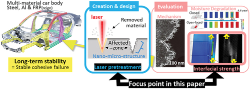
Figure 2. Properties and applications of mechanoluminescence (ML): (a) Comparison of simulation and ML image; (b) Raw and contour ML images during DCB test; (c) ML images during tensile test at various joints.
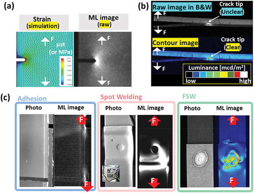
Figure 3. Laser surface pre-treatment. (a) Conditions and definitions; (b) Correlation of feed rate (Vf) and overlap ratio (OsR).
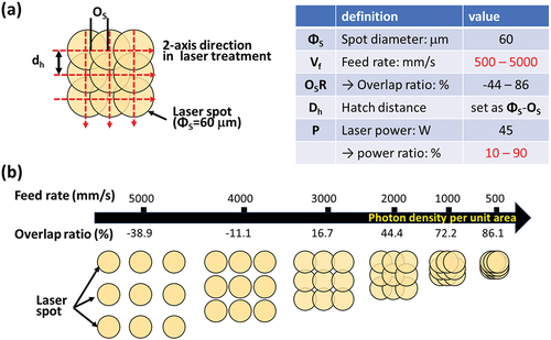
Figure 4. Schematic illustration of preparation flow for (a) Laser surface pre-treatment; (b) Adhesive bonding, and (c) Application of ML paint to SLS and DCB test specimens.
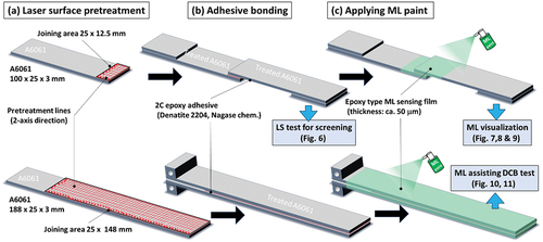
Figure 5. Picture and SEM images of laser treated surface of A6061 substrate for various combination of feed rate Vf (500–5000 mm/s) and laser power ratio (10–90%).
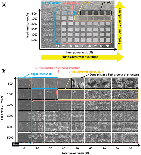
Figure 6. Results of SLS tests. (a) Plots of shear stress in 3D counter and 2D projection map; (b) List of shear stress values in average (N = 3) and photos of fracture surface.
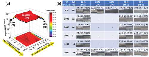
Figure 7. Observation of effect in adhesive thickness of SLS specimen for ML measurement. (a) Microscope observation of adhesive layer after adhesively bonding and (b) SEM images of laser-induced 3D micro-structure on aluminum (A6061) substrate.
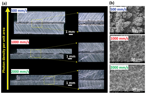
Figure 8. SLS test. (a) Schematic illustration of experimental set-up to identify the recording view of mechanoluminescence in ; (b) Plots of shear stress values and sum of thickness of residual adhesive layers on fracture surface; (c) Pictures of fracture surface and illustration of crack propagating behavior.
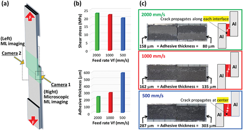
Figure 9. Visualization of dynamic strain distribution over time using ML microscopic images and ML images of adhesive joints obtained during SLS test using laser-treated aluminum substrates. Feed rate: (a) 500, (b) 1000, (c) 2000 mm/s. The red arrows indicate the interface between the two sides of the adhesive layer. White arrows with the F character indicates the load direction during tensile test.
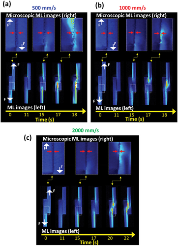
Figure 10. Results of DCB tests using laser-treated aluminum substrates. Feed rate: 500,1000, 2000, 3000, 40000 and 5000 mm/s. (a) R curves, (b) ML images for crack tip monitoring, (c) Comparison of fracture toughness values, (d) Photos of fracture surface, (e) Microscopic image and 2D profiles of fracture surface (vf = 500 and 2000 mm/s.) and (f) Their illustration regarding to crack propagation.
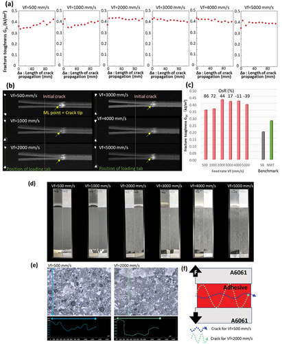
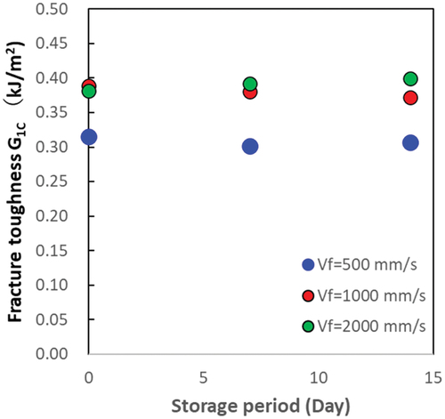
Figure 11. Effect of storage term on fracture toughness (G1C) after laser pretreatment to adhesive bonding. Storage condition.: ambient temperature and humidity, around 23°C and 40–50%RH, in air-conditioning condition.