Figures & data
Table 1. Publication names, authors, and websites of free GIS Books and information sources.
Figure 1. The GIS data framework is made up of both geometric properties and attributes associated with the geometry. A row in the attribute table exists for every polygon on the map. Some of the attributes for this Swiss layer include the names of cantons and their abbreviations, the country code, the country name and abbreviation, and the area. Reproduced with permission of Swisstopo (BA13016).
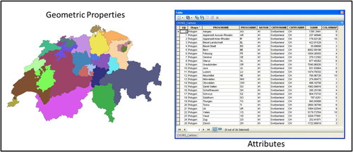
Figure 2. A map displaying a point, lines, and polygons. Reproduced with permission of Swisstopo (BA13016).
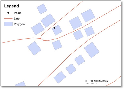
Figure 3. A map displaying the raster data structure of a landcover layer which was converted from vector format. The legend denotes the landcover properties which are displayed. Reproduced with permission of Swisstopo (BA13016).
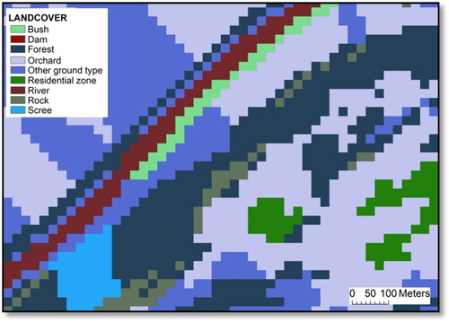
Table 2. Names, websites, and types of data available from some of the various free data sources.
Figure 4. A sample topographic map (scale 1: 200 000) covering the study area of Fribourg, Switzerland. This map comes from Swisstopo (Citation2013) and must only be used for visualization purposes in this paper. Reproduced with permission of Swisstopo (BA13016).
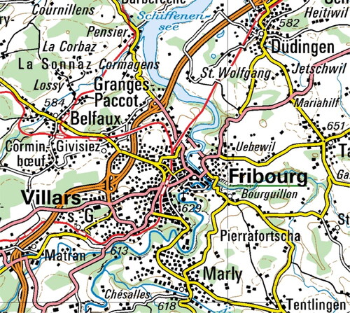
Figure 5. A sample orthophoto, with a resolution of 50 cm, showing the study area of Fribourg, Switzerland. This photo comes from Swisstopo (Citation2013) and must only be used for visualization purposes in this paper. Reproduced with permission of Swisstopo (BA13016).
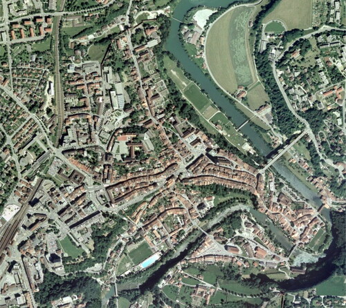
Figure 6. A section of the Swisstopo (Citation2013) Landsat image with a resolution of 25 m, covering the study area of Fribourg, Switzerland. Reproduced with permission of Swisstopo (BA13016).
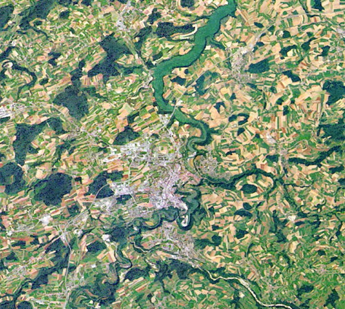
Figure 7. A sample digital elevation model (DEM) (30 m resolution) covering the study area of Fribourg, Switzerland. This map was a free download from ASTER GDEM which was projected to the Swiss projected coordinate system (CH1903 LV03).
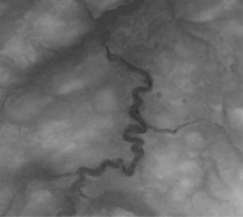
Figure 8. A map of the world shown in the WGS 84 geographic coordinate system.
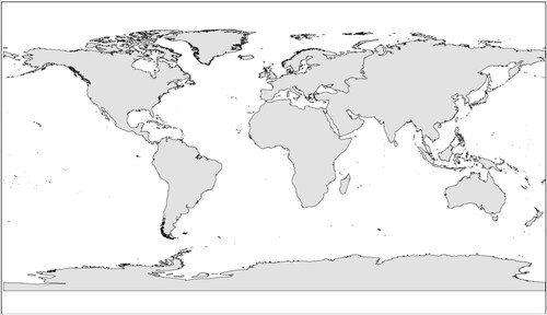
Figure 9. A map of the world shown in the CH 1903 projected coordinate system.
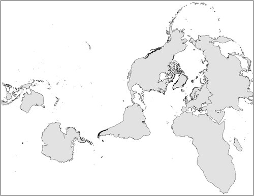
Figure 10. A map with the colony location point data, the DEM, and the county boundary layer displayed in ArcGIS. The symbology of the polygon layer has been changed to hollow polygons so the DEM is visible even though it is technically under the county layer.
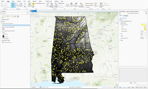
Figure 11. The pop-up dialog box displaying the results of clicking the screen using the Explore Cursor for all of the visible layers on the map. The results of the query show that the attributes of the clicked location, which was located in Lee County, AL. The remaining fields in the table are representative of those available in the attribute table.
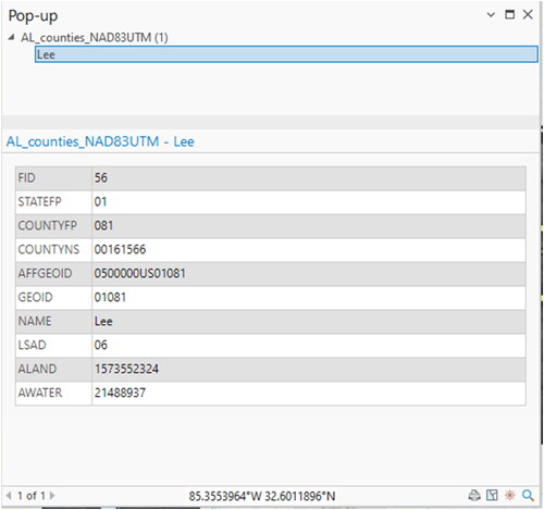
Figure 12. The select by attributes dialog box with the county layer as the input and the SQL builder and resulting equation shown. In this example, the equation will select all records in the table with the county number (countyfp) of 081 or 123.
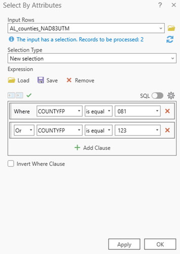
Figure 13. The results of the Select by Attributes query () are shown on the map and in the attribute table of the county boundary layer. The turquoise highlights represent all the selected data which represent Lee and Tallapoosa counties in Alabama.
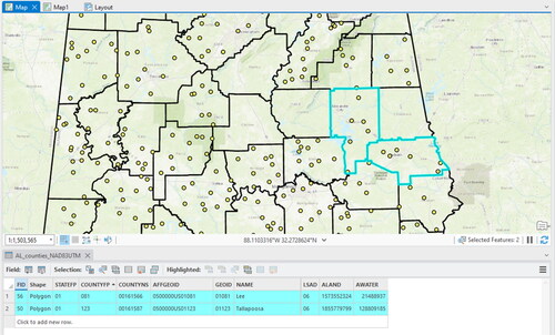
Figure 14. The select by location dialog box which shows that the features will be selected from the counties boundary layer where the layer intersects with the colony locations layer.
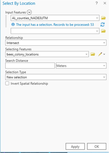
Figure 15. The results of the Select by Location query () which show the selected counties that intersect with colony locations, thus, all the county polygons with colony location points inside of them.
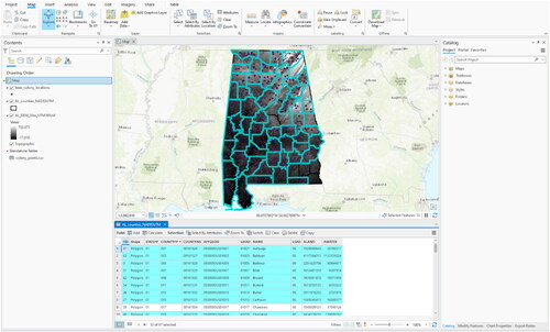
Figure 16. The results of exporting the selected data to a new shapefile. The new shapefile, colony_counties, depicts only the counties that have colonies inside them.
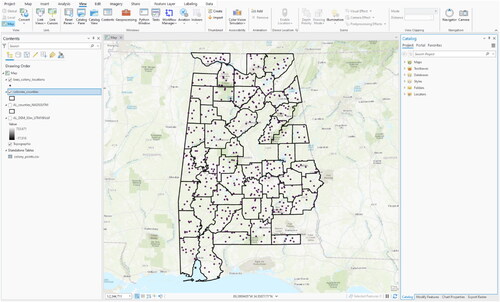
Figure 17. An example of table editing using the edit toolbar. Information has been added to the Apiary field of the colony locations point file by manually typing the information into the attribute table.
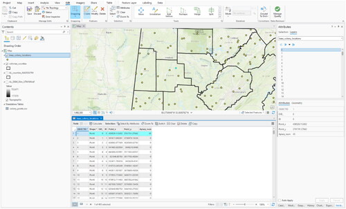
Table 3. Description of data types which are found in attribute tables, as well as the range of numbers or text they store and their uses. Adapted from the ArcGIS help menu (ESRI, Citation2013).
Figure 18. A visualisation of how the clip tool works in ArcGIS taken from the help menu (ESRI, Citation2013).
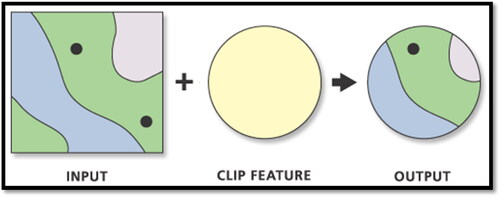
Figure 19. The dialog box of the intersect tool.
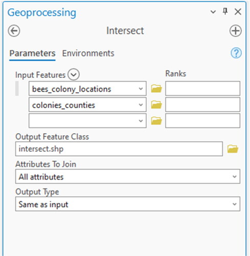
Figure 20. The attribute table showing the results of intersection between the bees_colony_locations and colony_communes layers.
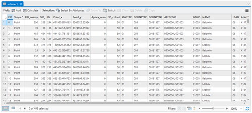
Figure 21. The dialog box of the buffer tool.
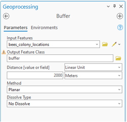
Figure 22. The resulting 2000 m buffers around each colony location.
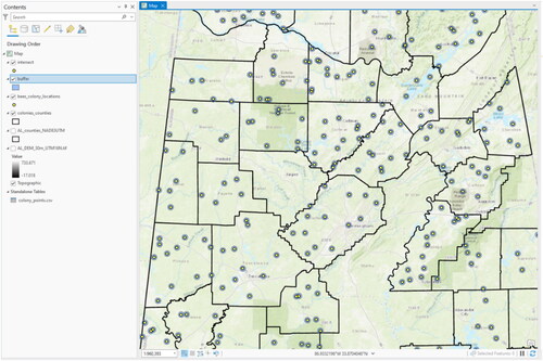
Figure 23. The dialog box of the multiple ring buffer tool.
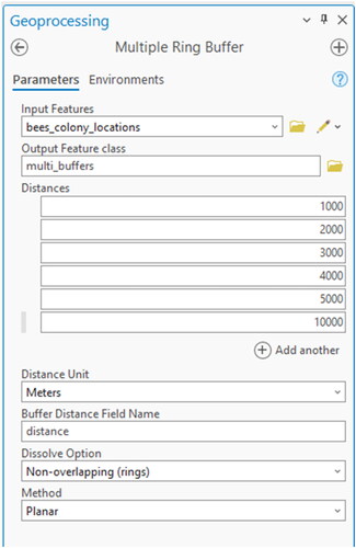
Figure 24. The resulting multiple ring buffers in 1000, 2000, 3000, 4000, 5000, and 10000 m increments around the colony locations.
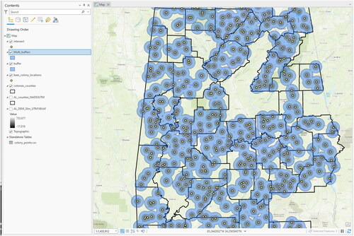
Figure 25. The dialog box of the dissolve tool.
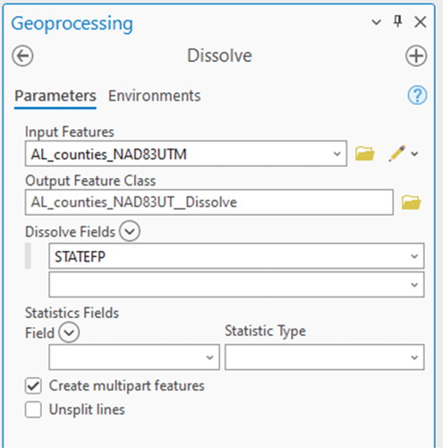
Figure 26. The results of the dissolving by the STATEFP attribute.
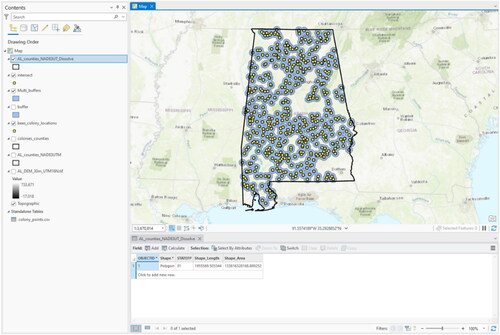
Figure 27. Dialog box of the project tool.
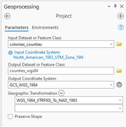
Figure 28. World Geodetic System (WGS 84) versus Universal Transverse Mercator North American Datum of 1983 (UTM NAD 83).
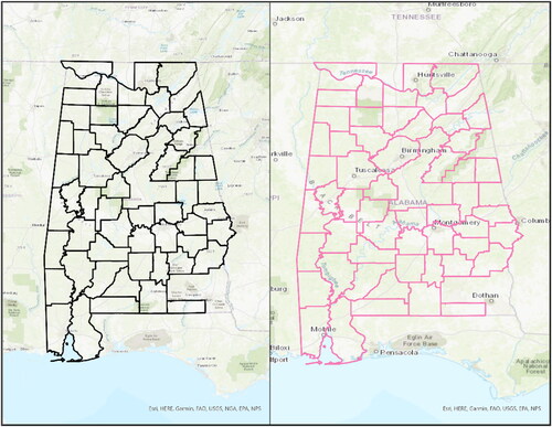
Figure 29. The layer to KML dialog box.
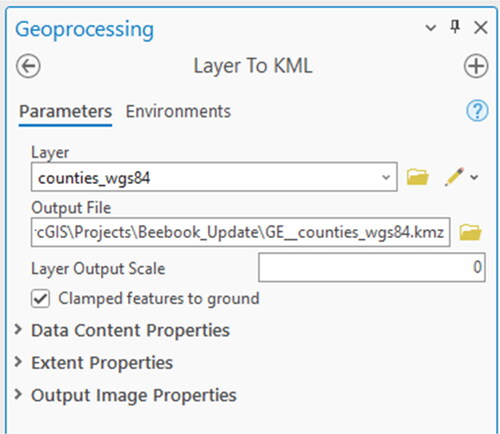
Figure 30. The results of Layer to KML tool imported into Google Earth.
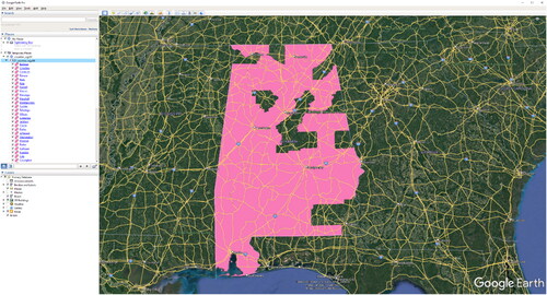
Figure 31. The slope tool dialog box.
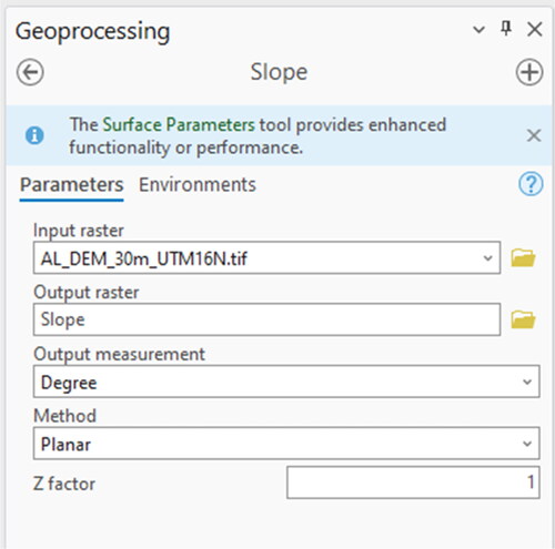
Figure 32. The result of slope calculation from the DEM.
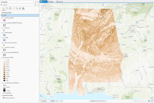
Figure 33. The symbol properties dialog box for the calculated slope layer.
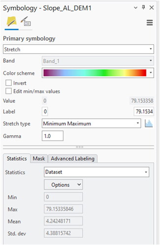
Figure 34. The results of changing the symbology of the slope layer.
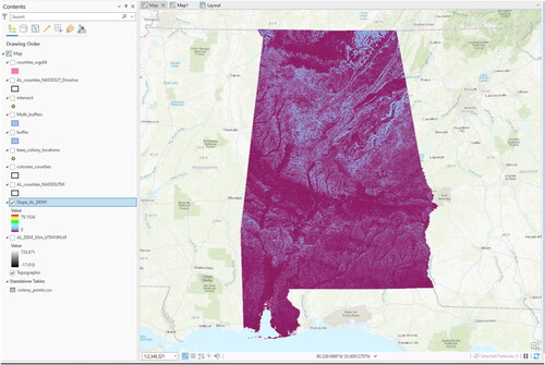
Figure 35. The aspect tool dialog box.
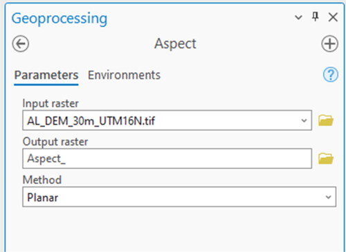
Figure 36. The result of the aspect calculation from the DEM.
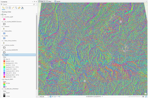
Figure 37. The Hillshade tool dialog box.
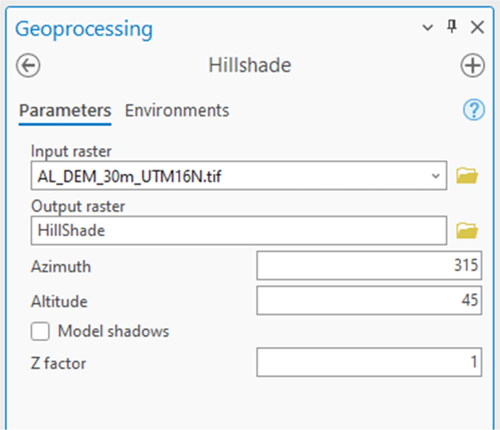
Figure 38. The result of the hillshade calculation from the DEM.
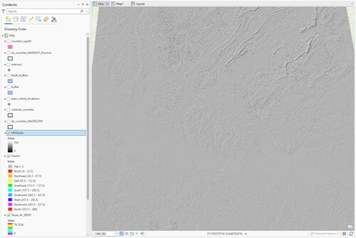
Figure 39. Example of a transparent DEM draped over the hillshade raster to show terrain definition.
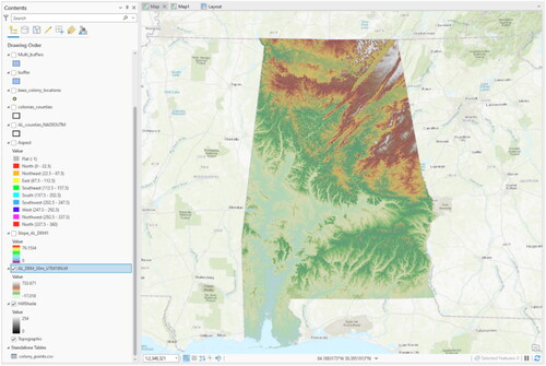
Figure 41. The result of the clip performed in . The land cover layer is now clipped to the extent of the Lee County layer.
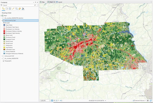
Figure 44. The results of the Zonal Statistics as Table calculation.
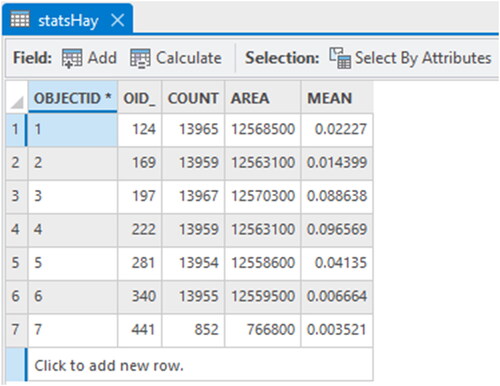
Figure 40. The dialog box from clipping the land cover data (nlcd_al_utm16.tif) layer to the extent of the Lee county layer.
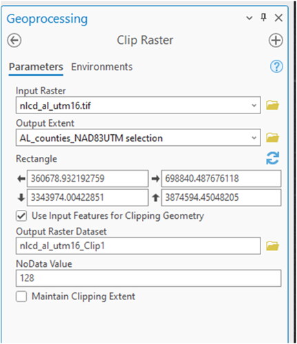
Figure 42. The Con Tool dialog box showing the equation used to select all of the Hay/Pasture land cover type from the entire raster.
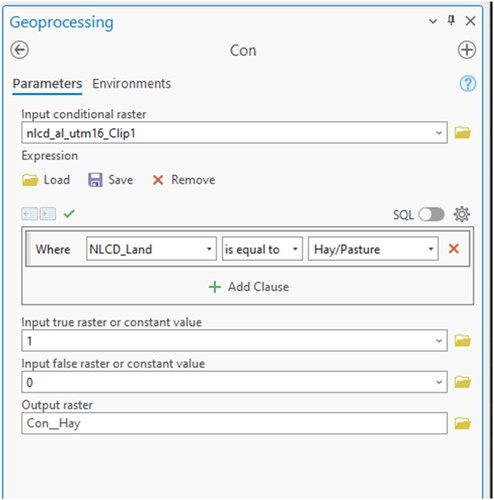
Figure 43. The Zonal Statistics as Table dialog box.
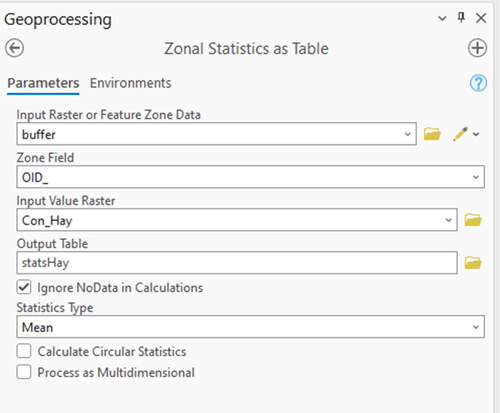
Figure 45. The Join Data dialog box.
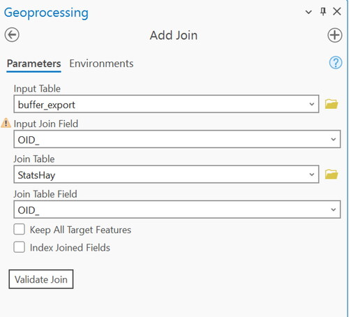
Figure 46. The Calculate Field dialog box used to create the “other” landcover classification in the buffer attribute table.
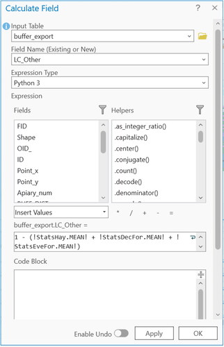
Figure 47. A sample graph created in ArcGIS Pro using the land cover statistics values.
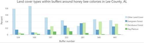
Figure 48. The results of symbolizing a layer based on the values of an attribute. In this example, each color represents a different county in Alabama.
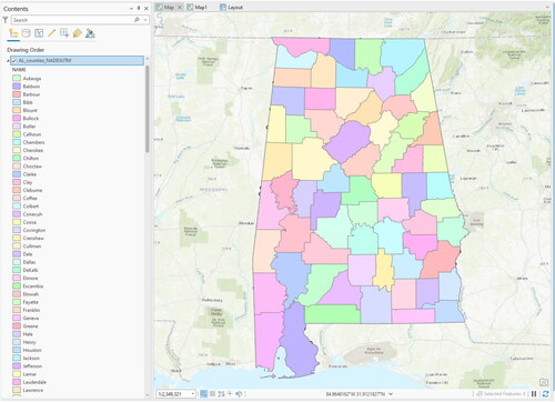
Figure 49. The result of turning the labels on for the AL_counties_NAD83UTM layer.
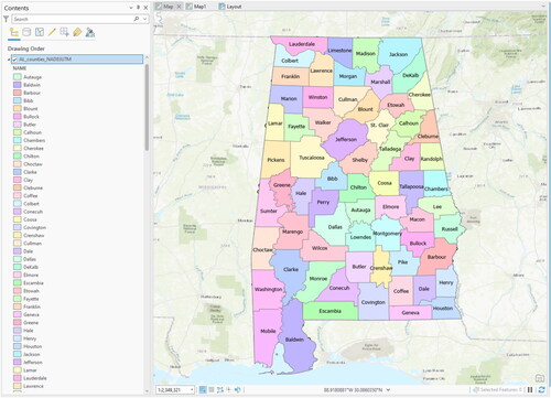
Figure 50. The creation of pie charts from the buffer layer properties symbology tab.
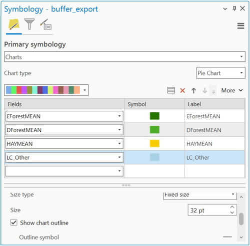
Figure 51. The resulting pie charts of the buffer areas shown on top of Lee County.
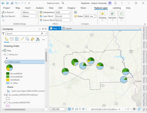
Figure 52. Example of a map layout.
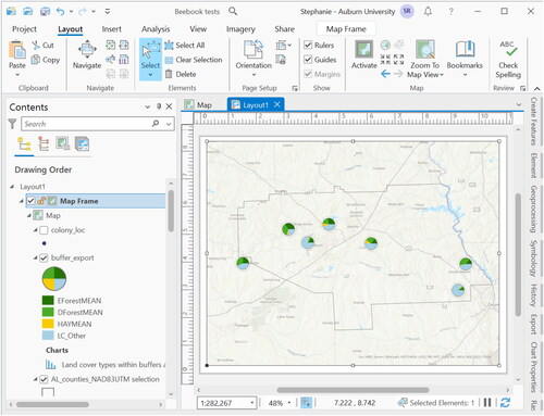
Figure 53. Final exported map.
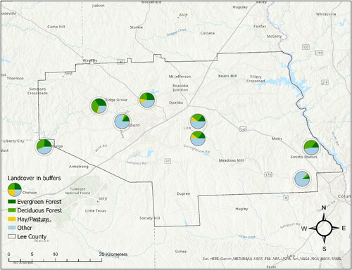
Figure 54. The graphical user interface of QGIS Desktop (version 3.22.6 “Białowieża”, running on Windows). The legend corresponds to the terms used in the official QGIS user Guide: Menu Bar (1), Tool Bar (2), Map Legend (3), Map View (4), Status Bar (5).
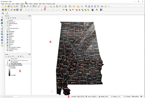
Figure 55. QGIS Browser serves as data manager. It can be added as a separate panel directly within QGIS Desktop.
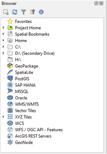
Figure 56. The QGIS Python Plugin Installer can be used to download and install additional program code from different repositories.
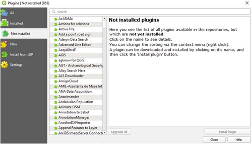
Table 4. QGIS plugins and repositories list used or mentioned in this tutorial.
Figure 57. The QGIS Plugin Manager can be used to enable (if they are already installed) or disable (without being uninstalled) plugins.
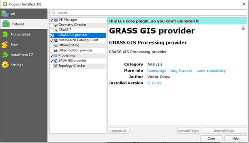
Figure 58. The Coordinate Reference System (CRS) of the project has to be defined within the Project Settings or Project Properties. On-the-fly CRS transformation is the default functionality in QGIS.
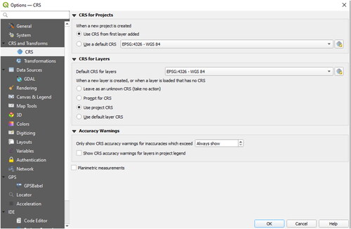
Table 5. The most important functions of the Manage Layers toolbar. This toolbar can be enabled and disabled by the main menu View > Toolbars > Manage Layers.
Figure 59. A polygon layer containing administrative districts (counties) for the state of Alabama has been loaded to the QGIS project.
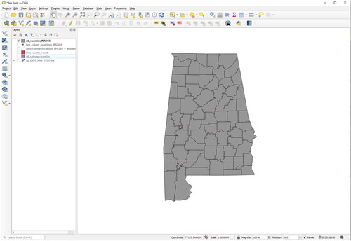
Figure 60. Result after adding the digital elevation model and zooming to its extent.
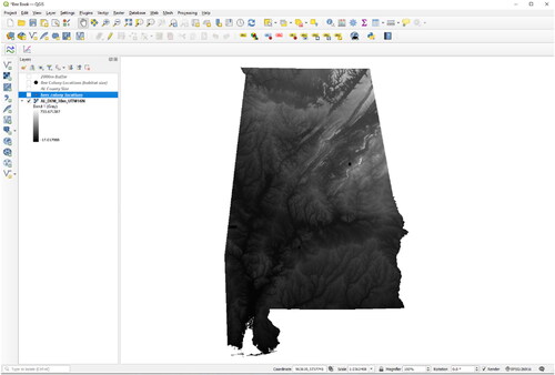
Figure 61. Create a Layer from delimited text files: By the use of coordinates stored in different columns of a delimited text file, point vector files can be created.
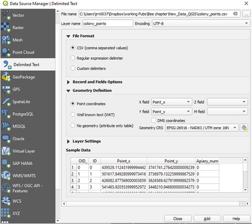
Figure 62. The map result after import of the honey bee colony locations (orange dots).
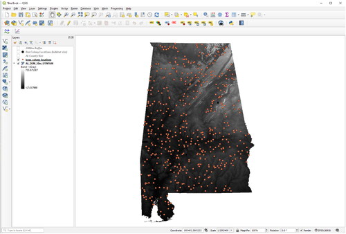
Figure 63. Dialog window to save an existing layer as a new vector layer. By the use of this function, file format conversions and even transformations between different coordinate reference systems are possible (defining the target CRS).
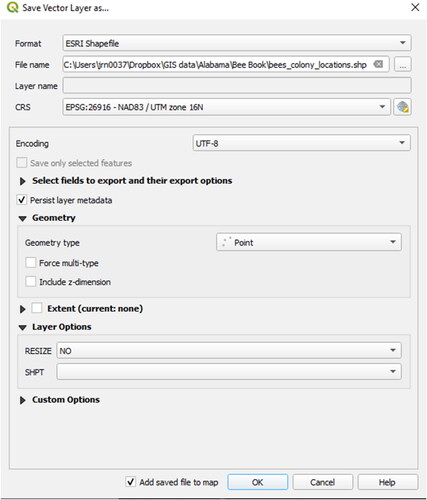
Figure 64. Save “Temporary Places” within Google Earth as KML-files to the file system.
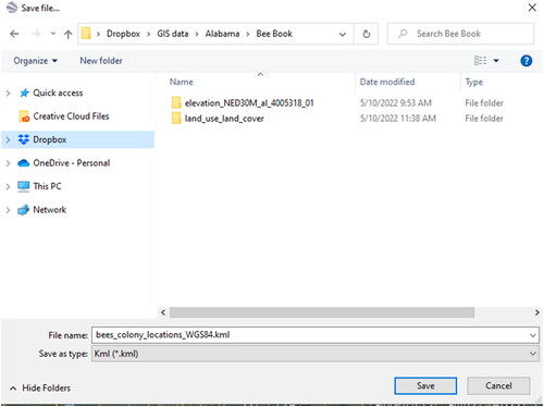
Figure 65. Information for the layer AL_counties_NAD83.shp in the Layer Properties.
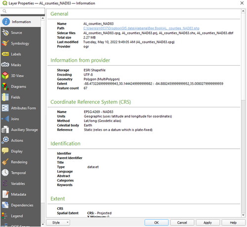
Figure 66. Symbol properties for QGIS vector layers. Different Symbol layer types can also be combined for more advanced visualization tasks (Button Add symbol layer)).
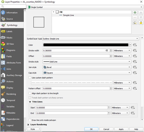
Figure 67. Result after performing a spatial query: The honey bee colonies are located within 53 different administrative districts around Alabama. The grey polygon represents the only county where no colonies are located.
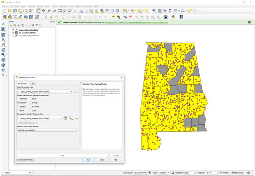
Figure 68. Selected features (one single feature corresponds to one table entry) within the Attribute table. All in all, the layer consists of 67 features.
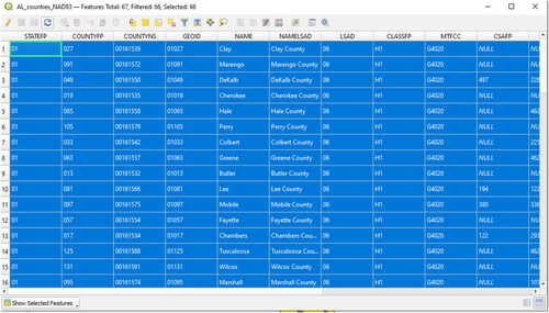
Figure 69. The Filter is used to restrict the features to those that meet the query (by the SQL where clause “COUNTYFP” = 081 OR “COUNTYFP” = 123).
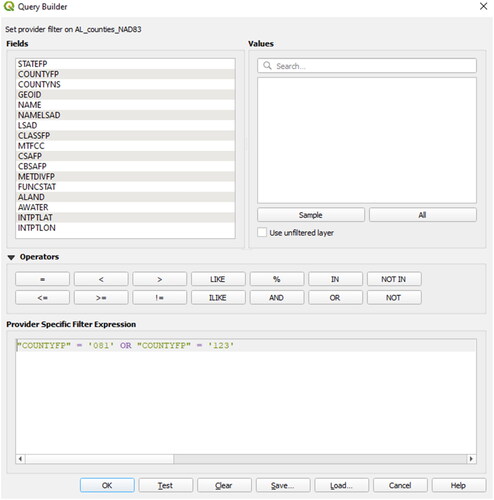
Figure 70. Result after the SQL Query is performed: There is only 4one polygon that meets the criteria of containing number 081 within the field “COUNTYFP”.
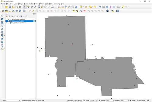
Figure 71. Save a selection to a new vector layer.
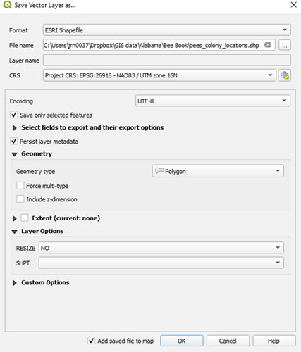
Figure 72. Editing attributes in QGIS.
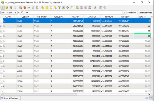
Table 6. The most important functions and the corresponding buttons for editing tasks.
Figure 73. Function Count Points in Polygon in QGIS.
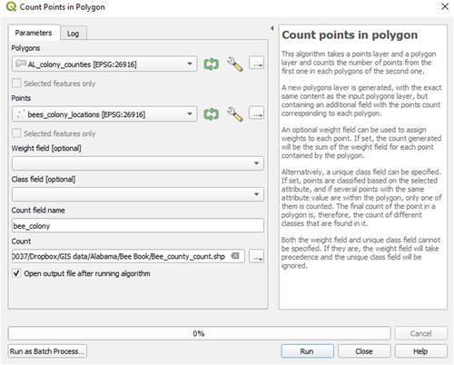
Figure 74. Calculate with attributes and geometrical statistics in the Field calculator.
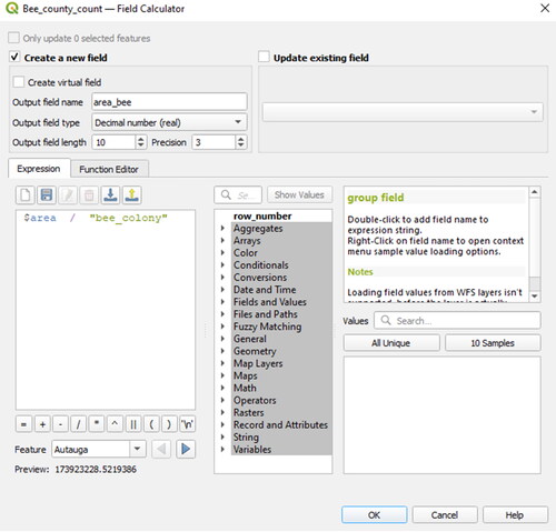
Figure 75. Add geometry columns to an existing or a new shapefile.
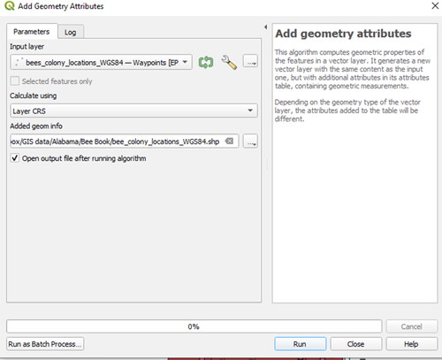
Figure 76. Vector to raster conversion using QGIS.
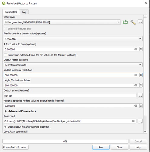
Figure 77. Symbolized raster image using five classes ranging from dark red (representing the county with the largest land area) to light red (representing counties with the smallest land area). In this case we set the Burn in Value to be ALAND which is the total area of the counties. Each pixel is symbolized using this value.
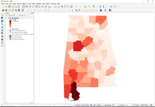
Figure 78. Raster to vector conversion using QGIS.
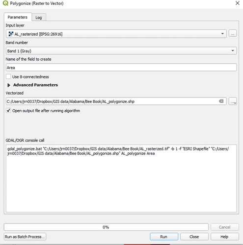
Figure 79. Project a raster dataset to a new target coordinate reference system (CRS).
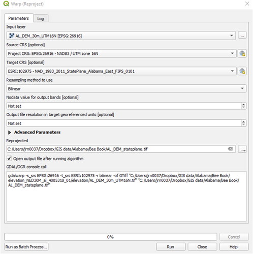
Figure 80. Adding a buffer of 2000 m to the honey bee colonies locations.
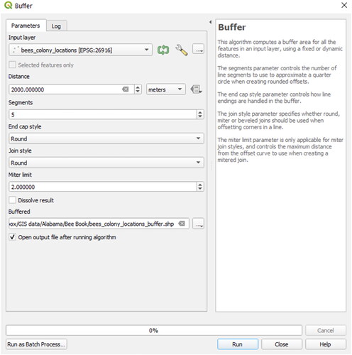
Figure 81. Clip the honey bee locations to the boundaries of Lee County.
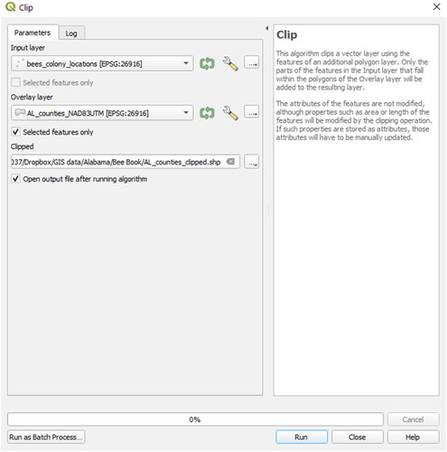
Figure 82. Using the Intersect Tool, overlapping areas are written to the resulting layer (the attributes of both original layers will be preserved).
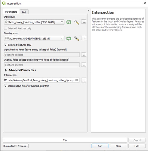
Figure 83. Dissolving polygons by the attribute “STATEFP”: The new layer will contain aggregated polygons based on this attribute.
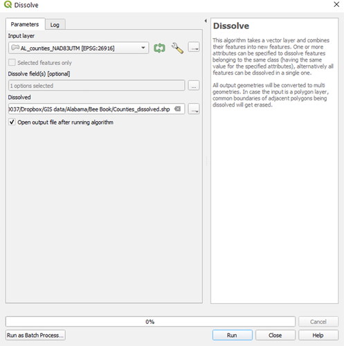
Figure 84. After applying the Dissolve tool, the polygon layer is transformed into a state outline (Blue). The white circles were created using a radial buffer of 2000 m around of all the honey bee colony locations.
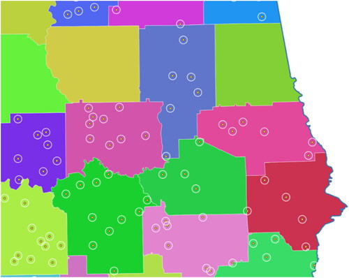
Figure 85. Attributes of a given layer can be attached to another by the use of a spatial join.
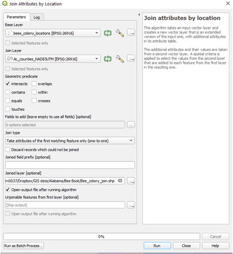
Figure 86. Basic statistics of a specific vector layer attribute field.
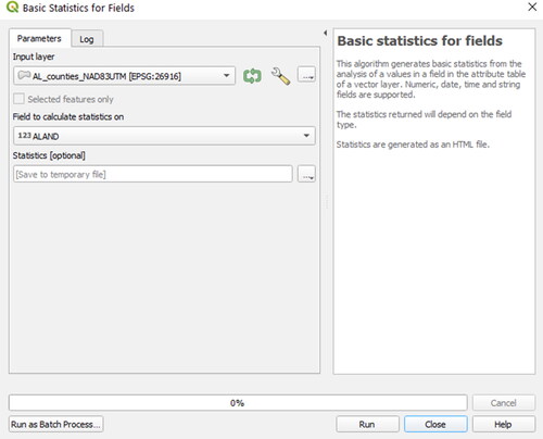
Figure 87. Calculating slope with QGIS.
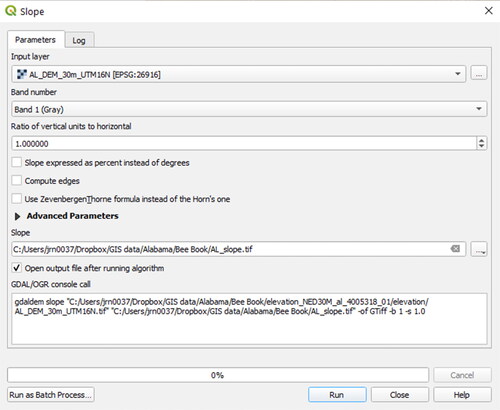
Figure 88. Calculating aspect with QGIS.
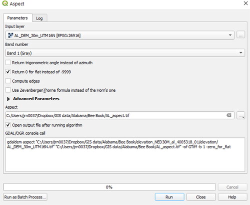
Figure 89. Hillshade tool to create shaded relief rasters based on a DEM.
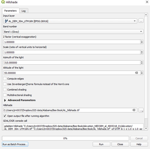
Figure 90. Compute elevation levels (isolines) based on a digital elevation model using the Contour function.
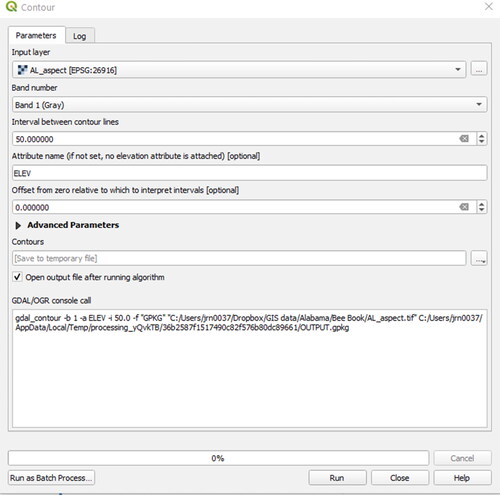
Figure 91. Compute mean coordinates from a point vector layer.
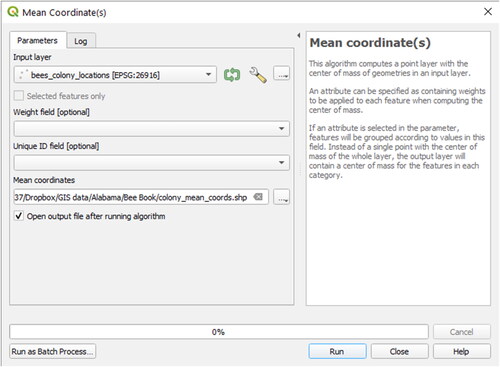
Figure 92. Output log from the point clustering nearest neighbour analysis.
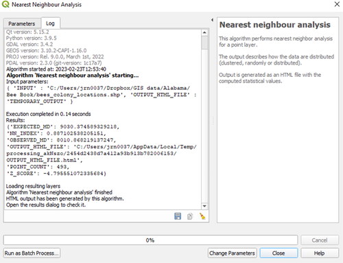
Figure 93. Generating a distance matrix between point vector layer(s).
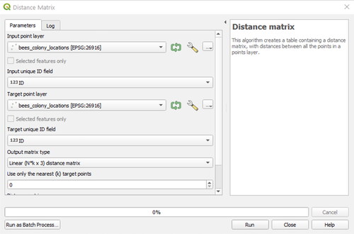
Figure 94. Spatial analysis computing the intersection between a DEM and an inclined plane with the QGIS plugin qgSurf.
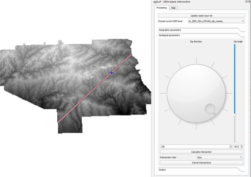
Figure 95. Raster information for the landcover dataset from Alabama.
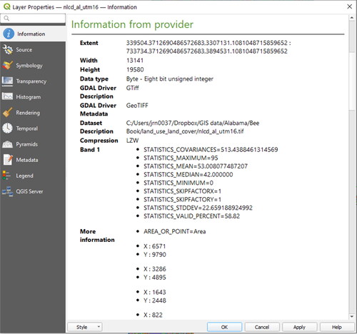
Figure 97. Intermediate result showing the counties and honey bee colonies on the Land Cover data set for the region within Lee County.
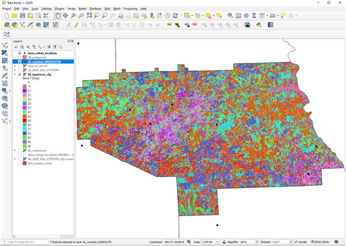
Figure 98. Setting the Colormap for the land cover data: for each integer value of the raster image a colour and a label is assigned.
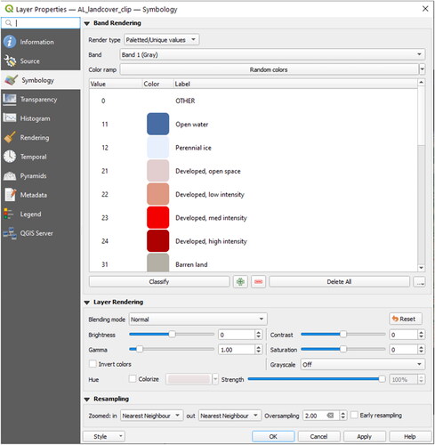
Figure 96. Clipping the Land Cover raster to the area of interest.
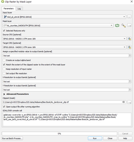
Figure 99. Separating bands of interest out of the Alabama Land Cover data set. The raster value 81 equals the land use category for “pasture/hay”.
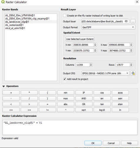
Figure 100. Performing zonal statistics from raster values based on a polygon vector layer.
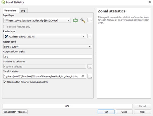
Figure 101. Visualising the percentage of different land cover categories within the honey bee buffers.
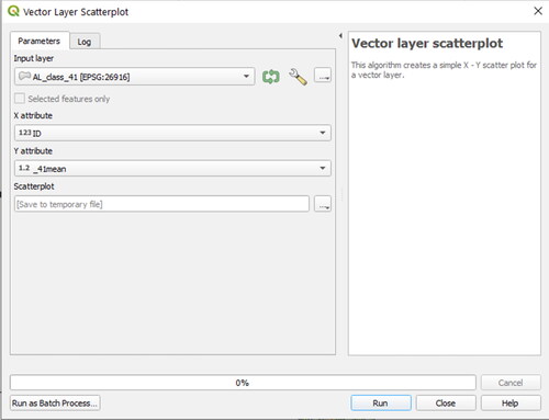
Figure 102. Calculate the percentage land use categories with the field calculator.
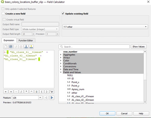
Figure 103. Join the zonal statistics output into the buffer layer.
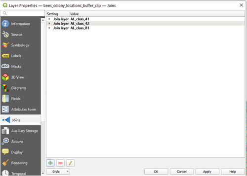
Figure 104. Setting labels based on attributes.
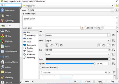
Figure 105. Creating diagrams based on layer attributes.
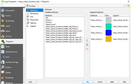
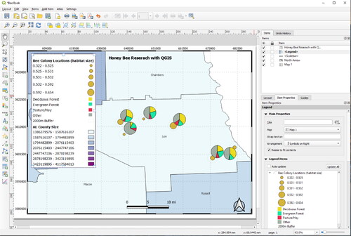
Figure 106. Map view after changing layer style properties and labelling options.
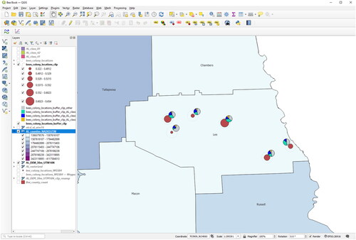
Figure 107. The QGIS print composer.

Figure 108. Final map with title, legend, north arrow, scale and coordinate grid in the QGIS print layout.