Figures & data
Figure 1. POD results of flow visualizations of a shallow cylinder wake. (a–d) The spatial modes . (e, f) The temporal coefficients
and
in black and
and
in grey. (g) Fourier power spectrum of the temporal coefficients
(black) and
(grey). The red dashed lines highlight the frequencies extracted using the DMD
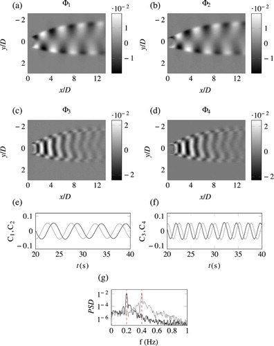
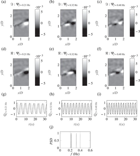
Figure 2. DMD results of flow visualizations of a shallow cylinder wake. (a–d) The real and imaginary components of the spatial modes and
respectively. (e, f) The real and imaginary temporal coefficients relating to
and
where the black line is the real component and the grey line is the imaginary component. (g) The Fourier power spectra of the temporal coefficients shown in (e) and (f).
(black) and
(grey)
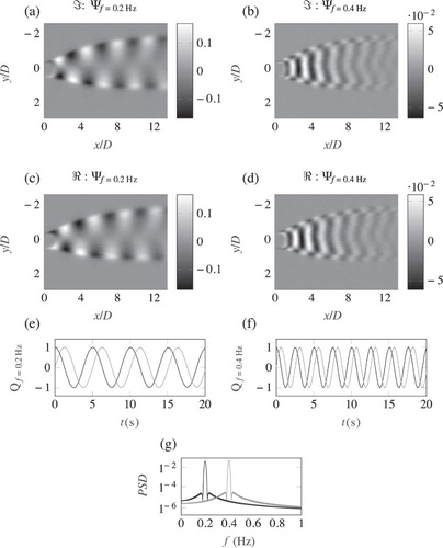
Figure 3. Illustration of the experimental set-up of the single groyne. Measurement section highlighted in white. (Not to scale.)
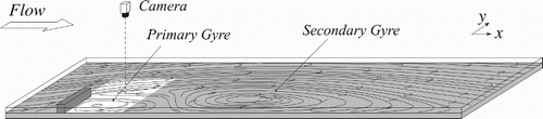
Figure 4. POD results of the near vorticity field of the shear layer generated by a lateral groyne in a shallow flow (groyne highlighted in white). (a) The time averaged vorticity field . (b, c) The POD spatial modes,
and
. (d, e) The POD temporal coefficients of
and
respectively, where the grey line denotes the mode which forms the conjugate pair. (f) The Fourier power spectra of the temporal coefficients shown in (d) and (e).
(black) and
(grey). The red dashed lines highlight the frequencies of importance; extracted using the DMD
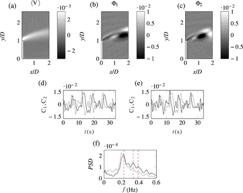
Figure 5. DMD results of the near vorticity field of the shear layer generated by a lateral groyne in a shallow flow. (a–f) The real and imaginary components of the DMD spatial modes ,
and
respectively. (g–i) The real and imaginary temporal coefficients relating to
and
, where the black line is the real component and the grey line is the imaginary component. (j) The Fourier power spectra of the temporal coefficients shown in (e) and (f).
(black),
(grey) and
(light grey)