Figures & data
Figure 1 Schematic plan view of experimental set-up for artificial partially vegetated case, showing low density (red) and high density (black and red) stem patterns
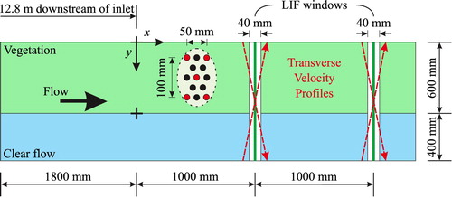
Figure 2 Experimental configurations for winter Typha (a, c) and summer Typha (b, d). (a) and (b) show details of the vegetation, illustrating the different stem densities for (a) winter φ = 0.01 and (b) summer φ = 0.019. (c) and (d) show the how the vegetation was cropped along the channel centreline, revealing the natural bed in the open channel region (right hand side)
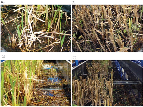
Figure 3 Transverse velocity and concentration profiles at Q = 3.4 × 10⁻³ m3 s−1 (left) and Q = 7.5 × 10⁻³ m3 s−1 (right) for (a, b) low-density artificial vegetation; (c, d) high-density artificial vegetation; (e, f) winter Typha; and (g, h) summer Typha
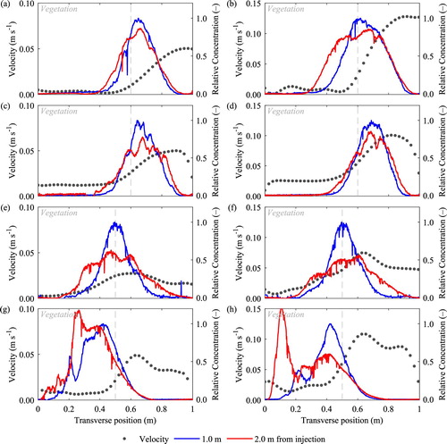
Figure 4 Comparison of model results (symbols) with analytical solutions (lines) for non-dimensional concentration, c*, where c* = c/cs1 and cs1 is the total mass flux at location x* = 1. (a) Rutherford (Citation1994) – uniform conditions – source at y* = 0.25 for U = 0.1 m s−1; Dy = 1 × 10⁻² m2 s−1, where w is channel width and (b) Kay (Citation1987) – step variation – source at y* = 1.0 for flow rate 2 × 10⁻³ m3 s−1; u1 = 0.1 m s−1; D1 = 1 × 10⁻² m2 s−1; with depth in y* > 0 twice that in y* < 0
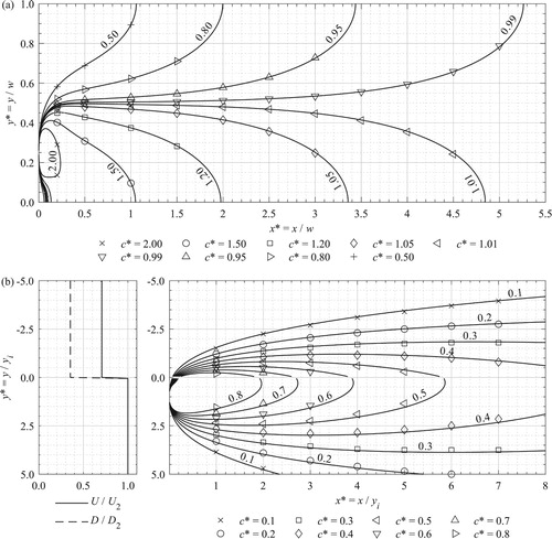
Figure 5 Assumed continuous dispersion coefficient distribution, illustrating values for D1, D2, DP, σ1 and σ2, where y* = y/y0, y0 indicates the location of the interface and y* < 1 is within vegetation
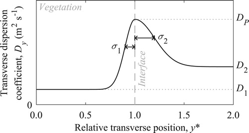
Figure 6 Comparison between optimized step (S) and continuous (C) distributions of dispersion coefficient (left) and predicted concentration profiles (right) for (a–d) low-density artificial vegetation, and (e–h) high-density artificial vegetation, where (a), (b), (e), and (f) are for Q = 3.4 × 10⁻³ m3 s−1 and (c), (d), (g), and (h) are for Q = 7.5 × 10⁻³ m3 s−1
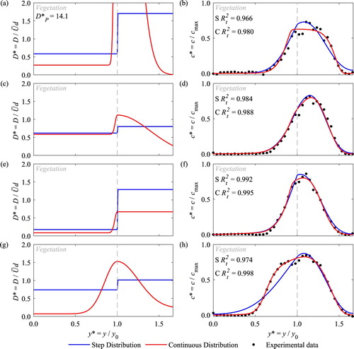
Figure 7 Comparison between optimized step (S) and continuous (C) distributions of dispersion coefficient (left) and predicted concentration profiles (right) for (a–d) Winter Typha, and (e–h) Summer Typha, where (a), (b), (e), and (f) are for Q = 3.4 × 10⁻³ m3 s−1 and (c), (d), (g), and (h) are for Q = 7.5 × 10⁻³ m3 s−1
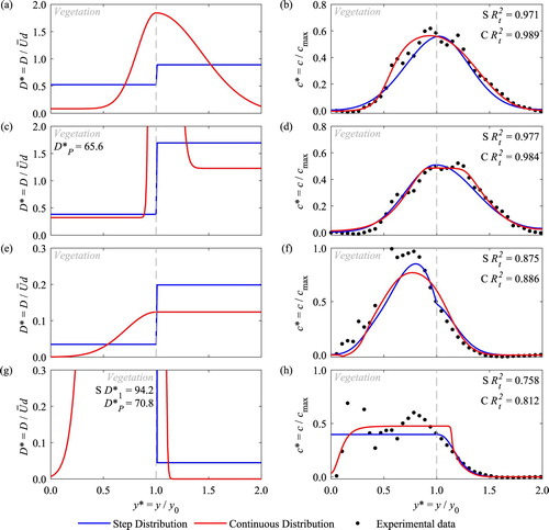
Table 1 Summary of goodness of fit,  , values between laboratory data and predicted spatial concentration profiles for step, continuous and estimated dispersion distributions
Figure 8 Comparison between optimized (filled) and estimated (open) continuous transverse dispersion coefficient distribution parameters with respect to flow rate
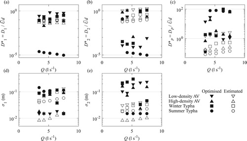
Figure 9 Estimated continuous velocity and transverse dispersion distributions (left), with resulting concentration profile compared with laboratory measurements (right), for (a, b) low-density artificial vegetation, and (c, d) high-density artificial vegetation, at Q = 7.5 × 10⁻³ m3 s−1 and for (e, f) winter Typha, and (g, h) summer Typha, at Q = 3.4 × 10⁻³ m3 s−1
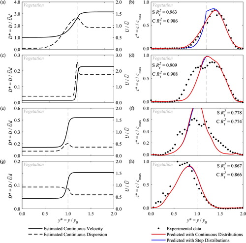
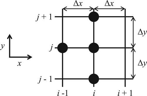
Figure A1 Location of computational grid points used to approximate Eq. (3) at node i, j