Role of low-order proper orthogonal decomposition modes and large-scale coherent structures on sediment particle entrainment

Figures & data

Figure 1 Experimental set-up and measurement system. Dimensions are in millimetre (mm)

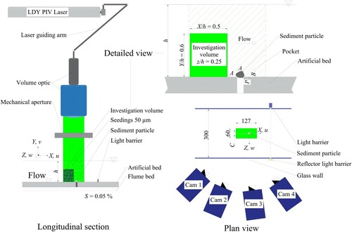
Table 1 Laser equipment and additional measurement characteristics

Parameter	Quantity
Laser	• LDY PIV laser (Double Cavity High Speed Laser, Litron)
	• 30 mJ output energy
	• 527 nm wavelength
	• 1000 Hz repetition rate
Four high-speed cameras	• Imager Pro HS 4M CMOS
	• Maximum repetition rate of 1300 Hz at max. resolution
	• Maximum resolution of 2016 × 2016 pixels
	• 12-bit digital output
	• Pixel size 11 µm
Timing Box	• PTU X High Speed
A/D electronic for external signals	• Type ADC-250-PCle
Calibration target	• La Vision Type 204-15
Lenses (#f)	• 16
Objectives	• 85 mm focal length (Zeiss)
Image Rate	• 0.8 kHz
Number of frames per camera	• 6123
Image Size	• 1488 × 1400 pixels
Size of laser volume X/Y/Z	• 127/120/60 mm
Flow seeding particles	• Polyamide particles
	• Diameter of 50 µm
	• Density of 1.016 g cm^−^3
Seeding density	• 0.04 ppp (particles per pixel)
Particle shift	• Maximum 10 voxels (three-dimensional pixel)
Light barrier	• Reflection light barrier Sick WL8

Figure 2 Summarized sediment particle entrainment tests. Triangles correspond to the mobilization tests, while the crosses correspond to the TOMO-PTV tests. Here h (cm) is the water depth and $\overline{h}$ (cm) the mean water depth of all conducted tests

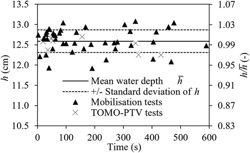
Table 2 Summary of the flow conditions, where Q is the discharge (l s⁻¹), h is the water depth (cm), U is the mean streamwise velocity (m s⁻¹), $\tau$ is the shear stress (N m⁻²), $u^{\ast }$ is the shear velocity (m s⁻¹), θ is the dimensionless Shields parameter and R_e* is the particle Reynolds number

	$Q$ (l s^−1)	$h$ (cm)	$U$ (m s^−1)	$\tau$ (N m^−^2)	$u^{\ast }$ (m s^−1)	θ (–)	Re* (–)
RF	19.6	12.6	0.52	0.336	0.0183	0.0031	217.6
S lower limit	19.6	12.3	0.53	0.331	0.0182	0.0030	216.1
S upper limit	19.6	12.7	0.51	0.337	0.0184	0.0031	218.0

Figure 3 Turbulence intensities normalized with the shear velocity $u^{\ast }$ of all tests (RF and 1S to 8S) measured with TOMO-PTV. Grey, red and blue symbols correspond to $〈{\sigma }_u〉/u^{\ast }$, $〈{\sigma }_w〉/u^{\ast }$ and $〈{\sigma }_v〉/u^{\ast }$, respectively. The symbols describe the conducted tests RF, 1S to 8S and are explained in the legend. The dashed lines correspond to the semi-theoretical curves of Nezu (1977)

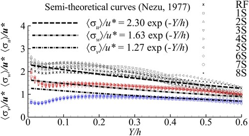
Figure 4 Cumulative TKE (a) and relative TKE (b) of the spatial POD modes for each test and the reference case. The symbols describe the conducted tests RF, 1S to 8S and are explained in the legend. A logarithmic scale is used

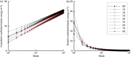
Figure 5 First temporal mode a₁ of the tests with sediment particle entrainment (a) 1S, (b) 2S, (c) 3S, (d) 4S, (e) 5S, (f) 6S, (g) 7S and (h) 8S. The dashed line marks the time of entrainment (te)

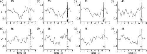
Figure 6 Summed turbulent kinetic energies (TKE) for the first five modes M (black lines) of the tests with sediment particle entrainment (a) 1S, (b) 2S, (c) 3S, (d) 4S, (e) 5S, (f) 6S, (g) 7S and (h) 8S. The grey shaded area shows the TKE contribution of only the first temporal mode M. The dashed line marks the time of entrainment (te)

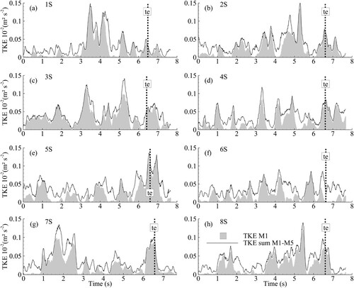
Table 3 TKE per temporal mode a_k in percent based on the cumulative energy of the first five modes at the time of sediment particle entrainment (te)

	1S	2S	3S	4S	5S	6S	7S	8S
a1,te	90.52	94.23	87.89	96.20	79.03	0.37	79.83	91.34
a2,te	0.61	0.93	10.66	0.17	18.06	27.03	1.66	3.56
a3,te	1.60	0.08	0.03	0.45	0.28	3.96	16.72	1.96
a4,te	7.20	4.00	1.32	3.18	0.10	65.78	1.65	2.35
a5,te	0.07	0.75	0.10	0.00	2.52	2.86	0.13	0.79

Table 4 Quadrant distribution in percent of the investigation volume for (i) Reynolds decomposed velocity vector fields (REY) and (ii) POD approximated velocity vector fields based on the first five modes for each test case at the time of sediment particle entrainment

	1S		2S		3S		4S		5S		6S		7S		8S
	REY	POD	REY	POD	REY	POD	REY	POD	REY	POD	REY	POD	REY	POD	REY	POD
QI	43.9	13.8	31.0	13.4	27.4	6.9	22.2	1.9	29.7	10.6	16.0	17.4	22.0	28.2	20.4	1.7
QII	4.9	0.0	0.3	0.0	6.7	0.0	1.4	0.0	4.0	0.9	27.6	58.9	0.1	0.1	0.7	0.2
QIII	2.5	0.9	0.3	0.0	3.0	0.0	2.9	0.0	1.0	0.0	31.6	6.2	0.0	0.0	0.3	0.2
QIV	48.8	85.2	68.4	86.6	62.9	93.1	73.5	98.1	65.3	88.5	24.8	17.6	77.9	71.7	78.6	97.9

Figure 7 Quadrants QII and QIV plotted as light grey spheres (indicating ejections) and dark grey squares (indicating sweeps); the TKE (m² s⁻²) based on the first five modes is plotted as black solid line in the investigation volume over the measurement period. Time of entrainment is marked with a vertical dashed line and labelled with te. The right vertical axis related to quadrants, describes the proportion of ejections QII and sweeps QIV in the investigation volume. (a) 1S, (b) 2S, (c) 3S, (d) 4S, (e) 5S, (f) 6S, (g) 7S and (h) 8S

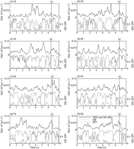
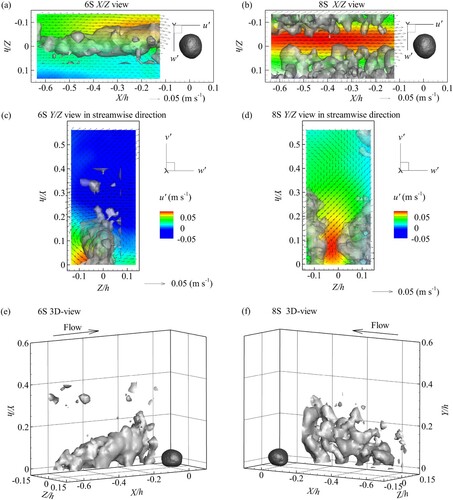
Figure 8 Comparison of the most TKE modes for test 6S and 8S. In case of 6S (a) the fourth spatial mode is shown and for test 8S (b) the first spatial mode. Flow direction is from left to right. Note that the reference vector in (a) is double the size of (b)

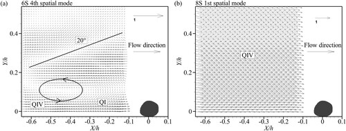
Figure 9 Comparison of the coherent structures based on the approximated vector fields between test 6S and 8S. Grey iso-surfaces correspond to the Qc = 1 (s⁻²) and the vectors correspond to the approximated fluctuating velocities. Horizontal plane at a height of half the particle diameter (a) and (b), vertical plane view in streamwise direction one particle diameter upstream of the sediment particle (c) and (d) and 3D view with the flow direction from left to right (e) and from right to left (f) are shown. (f) shows just one of the two observed structures for a better visibility. Contours in (a), (b), (c) and (d) show the turbulent streamwise velocity u’ in m s⁻¹. Note, that in (a), (b), (c) and (d) just every second vector is shown and a reference vector is given

Nezu, I. (1977). Turbulence structure in open channel flows (Ph.D. Thesis). Kyoto Univ., Kyoto, Japan. http://resolver.tudelft.nl/uuid:a41f39c2-fce6-4647-bd7a-1d412c720ed7

 Google Scholar