Figures & data
Table 1 Mechanical characteristics of the two domains comprising the coupled waveguide
Figure 1 (a) The white dashed frame encloses part of the DN80 HDPE pipe used in the experiment. (b) A bespoke 3D printed magnetic base is used to mount the transducer inside the pipe at approximately the pipe centre
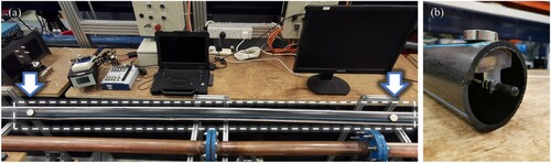
Figure 2 Signal path schematic of the experimental set-up: for the forward test, the probing signal is defined at the computer (1), converted from digital-to-analogue in the DAQ board (2), amplified (3) and emitted from the projector (4). Concurrently, a receiver (5) captures the system response, the signal is conditioned (6), converted from analogue-to-digital (7), and stored in the computer (1). For the second – time-reversed – part of the test, the transducer roles are interchanged: the receiver becomes the projector and vice versa, while the emitted signal is the stored response but time-reversed (first in, last out)
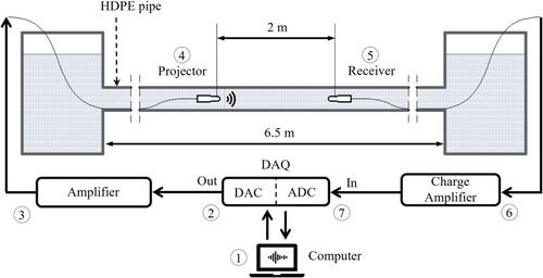
Figure 3 (a) A Gaussian modulated pulse is emitted from the source at one end of the pipe, with its amplitude spectrum shown in the inset. (b) The response of the system 2 m away from the source is characteristic of multipath propagation and comprises of two wavepackets, with the fastest attributed to the 1st radial, and the trailing to the 2nd radial mode
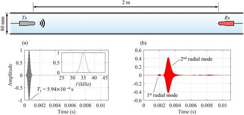
Figure 4 (a) The response of the system from the forward propagation test is time reversed and reemitted from the location of the original receiver. (b) the original pulse is successfully recreated at the location of the original source, albeit with the appearance of sidelobes
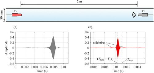
Figure 5 (a), (b) The time reversal test is repeated at a field-scale facility that employs a 250 m long DN150 HDPE pipe. The transducer set is placed 36.5 m apart, as dictated by the two access points “A” and “B” along a straight segment of the set-up
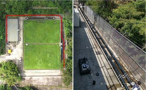
Figure 6 The experiment is repeated for a much larger waveguide with relative dimensions x/D = 248. (a) The source signal is a Gaussian modulated pulse of central frequency fc = 60 kHz, with its frequency content presented in the inset. (b) The system response is acquired at 36.5 m range and comprises of multiple wavepackets
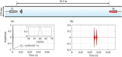
Figure 7 (a) The response of the DN150 HDPE pipe set-up from the forward test is time-reversed and emitted from the location of the original receiver. (b) The original pulse is recreated at the location of the original source and time t ≈ Ttot,2 – T2 displaying sufficient temporal compression
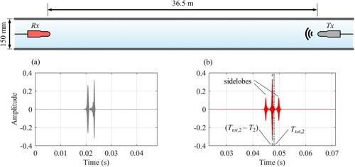
Figure 8 The time reversed pressure field is evaluated at multiple locations along the pipe. Here, the waveform at three locations is presented: 2 m (in blue), 1 m (in orange), and 3 m (in yellow) away from the time reversal source. The signal compresses and obtains its maximum amplitude 2 m from the time reversed source, coinciding with the location of the original source
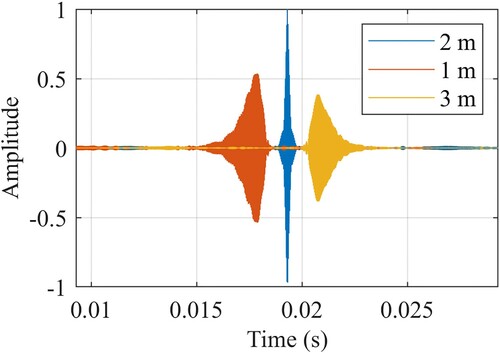
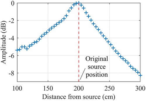
Figure 9 Multiple measurements are performed along the DN80 HDPE pipe at wavelength multiples to demonstrate spatial focusing. Maximum amplitude for the time reversed pressure field is observed at the location of the original source