Figures & data
Table 1 Levels of turbine and tidal flow models
Figure 1 Theoretical representation of the wake behind a single tidal turbine adopting (a) linear-momentum actuator disc theory where U denotes streamwise velocity, A area and p pressure with a subscript denoting location (adapted from Garrett & Cummins, Citation2013); and (b) Gaussian wake velocity field in which ΔU denotes velocity deficit, x distance downstream of the rotor, D rotor diameter and the wake width is represented by Dw with kw the wake expansion rate and ε · D the onset wake width
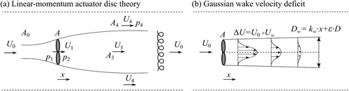
Figure 2 Interlink between physical scales of interest and available computational frameworks. The scales of resolved turbulence can range from those obtained with an eddy-viscosity model (EVM) in ocean or shallow water models to the sub-grid scales (SGS) in LES. Visualization of turbulent flow structures on the left subfigure follows from Ouro, Ramírez, et al. (Citation2019) and Ouro, Harrold, et al. (Citation2019).
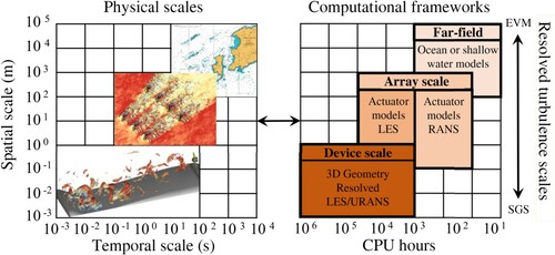
Figure 3 Simulation of a tidal stream turbine array with 12 turbines distributed in three rows. Comparison of the instantaneous streamwise velocity magnitude at hub height and on a vorticity iso-surface computed with RANS (left) using STREAM (Apsley et al., Citation2018) and from LES (right) using DOFAS (Ouro, Harrold, et al., Citation2019; Ouro, Ramírez, et al., Citation2019)
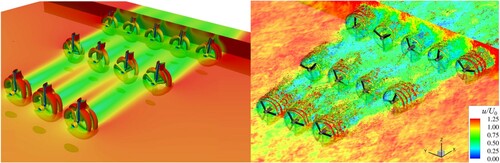
Figure 4 Left: bathymetry at Bluemull Sound (Scotland) depicting the location of the six tidal turbines and the computational domain modelled outlined with a dashed line. Right: LES results obtained with DOFAS (Ouro, Ramírez, et al., Citation2019) with values of instantaneous velocity and iso-surface of the vortex identification Q-criterion (Hunt et al., Citation1988)
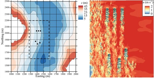
Figure 5 Instantaneous wake dynamics represented with Q-criterion iso-surfaces and contours of streamwise velocities, obtained from a LES using DOFAS (Ouro, Ramírez, et al., Citation2019)
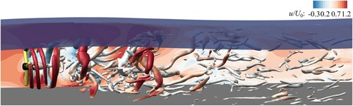
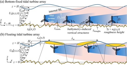
Figure 6 Schematic of the flow developed in tidal turbine arrays that are (a) bottom-fixed and (b) floating