A dynamical systems model of unorganized segregation

Figures & data

Figure 1. Schelling’s first example: linear tolerance schedules and their translation into the (W, B) phase plane.

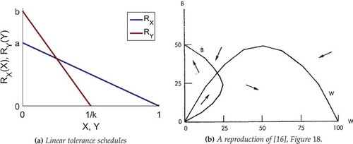
Figure 2. Equation (7) has three real roots in the colored area and one real root outside (and above the dotted line b = 1). The upper branch is the curve b = b+, which has a vertical asymptote at a = 4. The lower branch is the curve b = b − . The apex of the colored region is the point P: (a, b) = (ak, ab) = (3, 9). Below the dashed line b = 1, equation (7) has one real root Xe < 0. The color scale shows det(J) evaluated at the equilibrium point corresponding to the intermediate real root of equation (7), where this root exists.

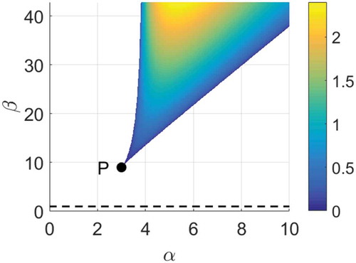
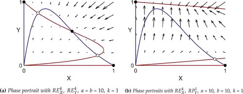
Figure 3. Phase portraits corresponding to different points in Figure 2. Stable equilibria are shown as filled circles and saddle points as open circles.

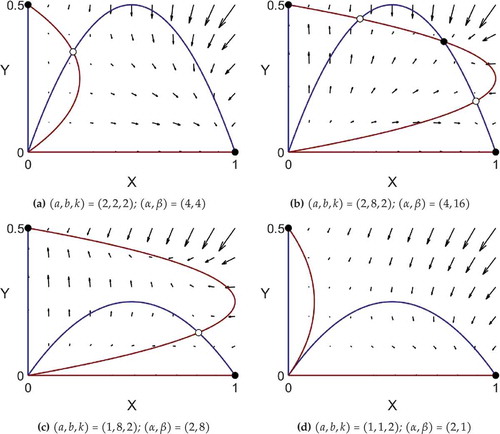
Figure 4. Bifurcation diagrams showing saddles (black) and stable nodes (green). At least one saddle point exists whenever b > 1.

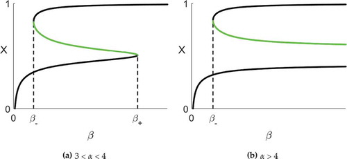
Figure 5. Blue regions correspond to the basin of attraction of X-only equilibrium (1, 0), and red regions to the basin of attraction of the Y-only equilibrium (0, 1k). White denotes the basin of attraction of the stable mixed state (integrated population mix) obtained from (7) when it exists.

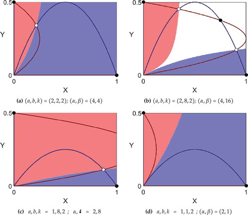
Figure 6. Limiting the X-population: The case when u < b4a and Z− < Z+ < Zu.

Figure 7. New population mixes can be created to the right of the blue curves, given by (19), by restricting the X-population and to the left of the red curves, given by (22), by restricting the Z-population. (a) The tolerance limits at the four points labelled (a), (b), (c), and (d) are shown in Figure 8. The black curves are from Figure 2. (b) Detail around the point P: (a, b) = (3, 9).

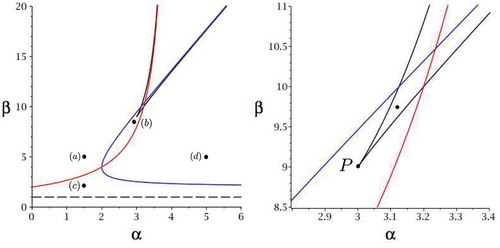
Figure 8. The tolerance limits at each of the four points (a), (b), (c), and (d) of Figure 7(a), with candidate cut-off values shown as a black dashed lines. Note that k = 2 in all four examples, and basins of attraction are colored as in Figure 5, with gray used to denote the basin of attraction of an additional stable mixed state.

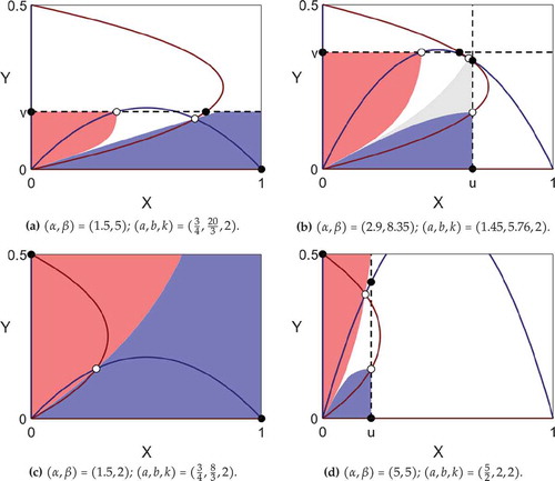
Figure 9. Phase portraits demonstrating that a globally more tolerant minority population can eliminate a stable mixed state.