Spontaneous cooperation for public goods

Figures & data

Figure 1. Cooperation for public goods. (a) Mean dissatisfaction $H/n$ and level of cooperation $M$. When all defect, $H/n$ is at a local minimum, on the left, but to proceed to the global minimum where all cooperate, on the right, participants are hindered by a hill. (b) Mean-field analysis with $S=\{1,-1/2\}$ shows below $T_c$ one stable state with mostly cooperators, at the top, and another stable state in finite time with mostly defectors, at the bottom. A metastable state in between, indicated by the dotted line, corresponds to the hilltop in Figure 1(a). Above $T_c$ only one state remains, where with increasing $T$, cooperators are joined by increasing numbers of defectors

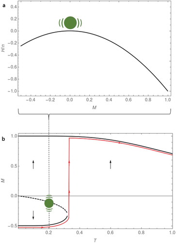
Figure 2. Numerical simulation on a university e-mail network with $n=1133$ and clustering $C=0.254$; data from Guimerà (2003). (a) the network at a near-critical turmoil level of $T=0.101$; $S=\{1,-1/2\}$. Some nodes start cooperating (red) whereas most still defect (blue). (b) $T_c$ is smaller than in the mean-field approximation, but the overall pattern is qualitatively the same (compare to Fig. 1 b)

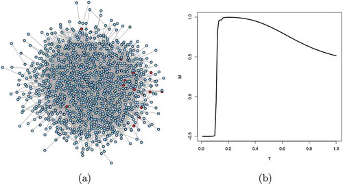
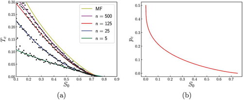
Figure 3. Consequences of shifting $S_0$ with the mean-field approach (MF), keeping $\mathrm{\Delta }=0.75$. (a) With increasing $S_0$, less agitation is necessary to turn defectors into cooperators. For comparison, numerical simulations on several random networks with density = 0.8 are shown as well. (b) The proportion of defectors $p_c$ at $T_c$ decreases with increasing $S_0$