Extremism, segregation and oscillatory states emerge through collective opinion dynamics in a novel agent-based model

Figures & data

Figure 1. An example of the interplay between agents’ thresholds, pairwise affinities, and pairwise influences. Panel (a) shows the evolving threshold ${\rho }_i$ of some agent $i$ as a function of $\parallel {\mathbf{v}}_i\parallel$, as per Equation (6)(6) ${\rho }_i(t)=\rho +(1-\rho )\left(1-e^{-\alpha \parallel {\mathbf{v}}_i(t)\parallel }\right).$(6) , with reinforcement rate $\alpha =0.1,0.2,0.4,0.8$. Panels (b-e) are snapshots of the connections among four agents with two-dimensional opinions $(0,0),(1,0),(1,1)$ and $(0,1)$ which we assume, for this illustration, have been held fixed for at least $\mu$ time-steps. The arrows denote the three distinct types of pairwise influence. The numbers that annotate the arrows are the pairwise affinities calculated by Equation (1)(1) $a_{ij}(t)=\frac{1}{{\left(1+{\sum }_{\tau =0}^{t}w(\tau ;t,\mu ){∥{\mathbf{v}}_j(\tau )-{\mathbf{v}}_i(\tau )∥}^2\right)}^{1/2},}$(1) to 3dp precision. Panels (b,c) have universal threshold ${\rho }_i=0.5$ for all $i$; panels (d,e) have evolving thresholds with baseline $\rho =0.5$ and reinforcement rate $\alpha =0.2$, calculated by Equation (6)(6) ${\rho }_i(t)=\rho +(1-\rho )\left(1-e^{-\alpha \parallel {\mathbf{v}}_i(t)\parallel }\right).$(6) to 3dp precision. The memory capacity is $\mu =1$ in (b,d) and $\mu =2$ in (c,e).

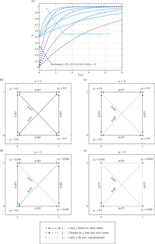
Table 1. Parameters used in numerical simulations.

Parameter	Values used
$D$ (Dimensionality of every opinion)	1, 2, 3, 5
$\mu$ (Memory capacity of population)	2, 10
$\rho$ (Universal threshold in Section 3.2; baseline threshold in Section 3.3)	0, 0.01, 0.02, $\dots$, 0.99
$\alpha$ (Reinforcement rate; only in Section 3.3)	0.1, 0.2, 0.4, 0.8

Figure 2. Examples of one- and two-dimensional opinion trajectories of $N=100$ agents evolving according to (3), with memory capacity $\mu =2$. Panels (a,b): One-dimensional dynamics from a common initial state (sampled from a standard normal distribution), with different universal thresholds: $\rho =0$ (a) and $\rho =0.8$ (b). Panels (c,d): Two-dimensional dynamics from a common initial state (the two dimensions sampled from two independent standard normal distributions), with different universal thresholds: $\rho =0$ (c) and $\rho =0.8$ (d); $v^{(1)}$ and $v^{(2)}$ denote the first and second dimensions of the opinions, respectively. Consensus is reached in (a,c), while (b) exhibits segregation with 6 distinct clusters, and (d) shows segregation with 9 distinct clusters.

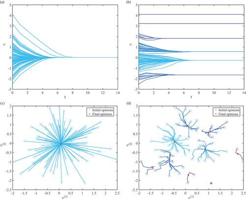
Figure 3. Evolution of the connectome of the population as the opinions evolve in the manner of Figure 2d, with parameters $D=2,\mu =2,\rho =0.8,\alpha =0$. Opinions are represented by (blue) dots while connections between agents are (black) lines. The opacity of the dots increase as agents overlap, so that the larger the cluster, the darker the dots. Since the threshold $\rho$ is universal, every connection is bidirectional: the pair of agents influence each other. The opacity of the dots increase as agents overlap, so that the larger the cluster, the darker the dots.

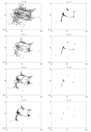
Figure 4. Evolution of the connectome of the population as the 2-dimensional opinions evolve from the same initial state as in Figure 2d, with parameters $\mu =10,\rho =0.8,\alpha =0$. Opinions are represented by (blue) dots while connections between agents are (gray) lines. The opacity of the dots increase as agents overlap, so that the larger the cluster, the darker the dots. Since the threshold $\rho$ is universal, every connection is bidirectional: the pair of agents influence each other.

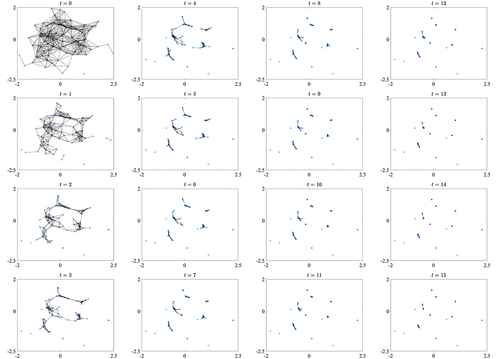
Figure 5. Number of clusters formed for $N=100$ agents with universal threshold $\rho$ taking values as per Table 1; 1000 simulations per value of $\rho$. A common set of 1000 initial states are used. Dimensionality $D=$ 1 (a,b), 2 (c,d), 3 (e,f), and 5 (g,h). Memory capacity $\mu =$ 2 (a,c,e,g), and 10 (b,d,f,h).

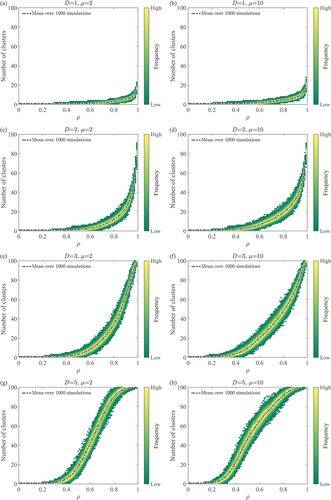
Figure 6. Convergence time for $N=100$ agents with universal threshold $\rho$ taking values as per Table 1; 1000 simulations per value of $\rho$. A common set of 1000 initial states are used. Dimensionality $D=$ 1 (a,b), 2 (c,d), 3 (e,f), and 5 (g,h). Memory capacity $\mu =$ 2 (a,c,e,g), and 10 (b,d,f,h).

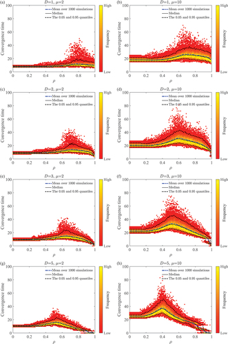
Figure 7. Opinion drift for $N=100$ agents with universal threshold $\rho$ taking values as per Table 1; 1000 simulations per value of $\rho$. A common set of 1000 initial states are used. Dimensionality $D=$ 1 (a,b), 2 (c,d), 3 (e,f), and 5 (g,h). Memory capacity $\mu =$ 2 (a,c,e,g), and 10 (b,d,f,h). The grouping precision of opinion drift is 0.001; that is, the histogram bins are the intervals $[0,0.001),[0.001,0.002)$, and so on.

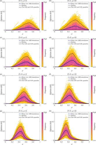
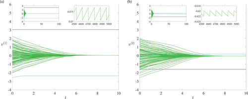
Figure 8. Under evolving heterogeneous thresholds, with reinforcement rate $\alpha >0$, a small number of simulations out of the total 1000 fail to produce a steady state. That number, $F_{\mu ,\alpha }(\rho )$, depends on $\alpha$, the memory capacity $\mu$, and the baseline threshold $\rho$. Panel (a): $(D,\mu )=(2,2)$. Panel (b): $(D,\mu )=(2,10)$.

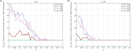
Figure 9. Under evolving heterogeneous thresholds, the mean number of clusters formed (a,b) and the mean convergence time (c,d) are taken, for each parameter setting $(\mu ,\alpha ,\rho )$, from all simulations that result in steady states. Panels (a,c): $\mu =2$. Panels (b,d): $\mu =10$. Other parameters used for each panel: $D=2$, $\alpha =0.1,0.2,0.4,0.8$, and $\rho =0,0.01,0.02,\dots ,0.99$.

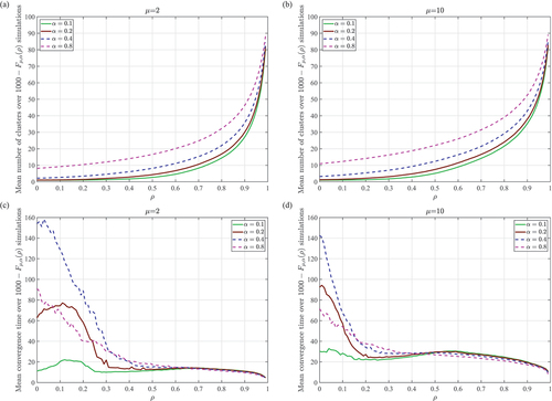
Figure 10. Two examples of collective drift of opinions under evolving heterogeneous thresholds. The first and second dimensions of the opinions are denoted by $v^{(1)}$ and $v^{(2)}$, respectively. Drifting begins at some $t$ which is chosen to best illustrate the trajectory (rather than rigorously defined). Final opinions are taken at the convergence time, $t_c$. Parameters: $\mu =2,\rho =0,\alpha =\mathrm{0.8.}$

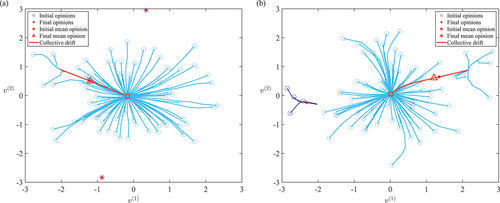
Figure 11. Key steps in the evolution of the connectome of the population as the opinions evolve in the manner of Figure 10a, with parameters $D=2,\mu =2,\rho =0,\alpha =0.4$. Opinions are represented by (blue) dots, bidirectional connections are dark (gray) lines and unidirectional connections are light (blue) lines. The opacity of the dots increase as agents overlap, so that the larger the cluster, the darker the dots. Since the threshold $\rho$ is heterogeneous, unidirectional connections may exist, where agent $j$ influences agent $i$ without reciprocation.

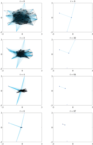
Figure 12. Extremisation measure for $N=100$ agents with evolving heterogeneous thresholds ${\rho }_i(t)$; the baseline threshold $\rho$ takes values as per .Table 1. A thousand simulations are performed per value of $\rho$ and a common set of 1000 initial states are used for each $\rho$. Dimensionality $D=2$. Memory capacity $\mu =$ 2 (a,c,e,g), and 10 (b,d,f,h). Reinforcement rate $\alpha =$ 0.1 (a,b), 0.2 (c,d), 0.4 (e,f), and 0.8 (g,h). The grouping precision of extremisation measure is 0.01; that is, the histogram bins are intervals of size 0.01, giving the same number of bins as in Figure 7.

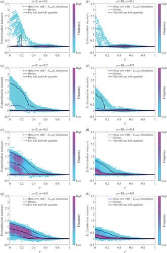
Figure 13. Example of a system that fails to reach a steady state under evolving heterogeneous thresholds. The time periods 0–10, 0–100, and 4500–5000 are shown. In particular, the top-right inset in each panel shows only the large-time dynamics of the oscillatory cluster. Panels (a,b) show the first and second dimensions of the opinions, respectively. Each cluster is shown in a different color. Parameters: $D=2,\mu =2,\rho =0,\alpha =0.4$.